Recognizing and Learning Object Categories Based on work and slides - - PowerPoint PPT Presentation

1

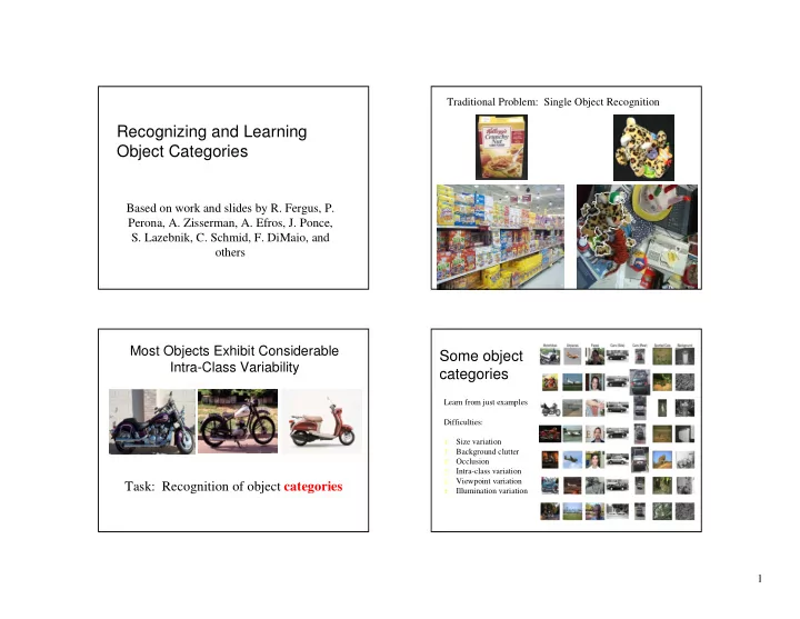
Recognizing and Learning Object Categories

Based on work and slides by R. Fergus, P. Perona, A. Zisserman, A. Efros, J. Ponce,

• S. Lazebnik, C. Schmid, F. DiMaio, and
• thers

Traditional Problem: Single Object Recognition

Most Objects Exhibit Considerable Intra-Class Variability Task: Recognition of object categories

Some object categories

Learn from just examples Difficulties: f Size variation f Background clutter f Occlusion f Intra-class variation f Viewpoint variation f Illumination variation

2

Chairs

Related by function, not form

Approach 1: Discriminative Methods

Object detection and recognition is formulated as a classification problem

Bag of image patches

Decision boundary

… and a decision is taken at each window about if it contains a target object or not

Computer screen Background

In some feature space

Where are the screens?

The image is partitioned into a set of overlapping windows

HRCT Lung Image

Dilated bronchus

Training Examples

• ×

3 § Formulation: binary classification

Formulation

+1

• 1

x1 x2 x3 xN

… …

xN+1 xN+2 xN+M

• 1
• 1

? ? ? …

Training data: each image patch is labeled as containing the object or not Test data Features x = Labels y = Where belongs to some family of functions

• Classification function
• Minimize misclassification error

(Not that simple: we need some guarantees that there will be generalization)

Discriminative Methods

106 examples

Nearest Neighbor Shakhnarovich, Viola, Darrell 2003 Berg, Berg, Malik 2005 … Neural Networks LeCun, Bottou, Bengio, Haffner 1998 Rowley, Baluja, Kanade 1998 … Support Vector Machines and Kernels Conditional Random Fields McCallum, Freitag, Pereira 2000 Kumar, Hebert 2003 … Guyon, Vapnik Heisele, Serre, Poggio, 2001 …

Object categorization: Object categorization: the statistical viewpoint the statistical viewpoint

) | ( image zebra p

) ( e zebra|imag no p

vs.

§ Bayes’s rule: ) ( ) ( ) | ( ) | ( ) | ( ) | ( zebra no p zebra p zebra no image p zebra image p image zebra no p image zebra p ⋅ =

posterior ratio likelihood ratio prior ratio

Object categorization: Object categorization: the statistical viewpoint the statistical viewpoint

) ( ) ( ) | ( ) | ( ) | ( ) | ( zebra no p zebra p zebra no image p zebra image p image zebra no p image zebra p ⋅ =

posterior ratio likelihood ratio prior ratio

§ Discriminative methods model the posterior § Generative methods model the likelihood and prior

4

Discriminative

§ Direct modeling of

Zebra Non-zebra Decision boundary

) | ( ) | ( image zebra no p image zebra p § Model and

Generative

) | ( zebra image p

) | ( zebra no image p

Middle Low High Middle Low

) | ( zebra no image p ) | ( zebra image p

Three main issues Three main issues

§ Representation

§ How to represent an object category

§ Learning

§ How to form the classifier, given training data

§ Recognition

§ How the classifier is to be used on novel data

Constructing models of image content

Basic components: local features and spatial relations

Textures Objects Scenes

5

Constructing models of image content

Basic components: local features and spatial relations

Textures Objects Scenes Local model

Constructing models of image content

Basic components: local features and spatial relations

Textures Objects Scenes Local model

Constructing models of image content

Basic components: local features and spatial relations

Textures Objects Scenes Local model Semi-local model

Constructing models of image content

Basic components: local features and spatial relations

Textures Objects Scenes Local model Semi-local model

6

Constructing models of image content

Basic components: local features and spatial relations

Textures Local model Objects Semi-local model Scenes Global model

(usually appearance)

Approach 2: Generative Methods using Bag of Words Models

§ An image is represented by a collection of “visual words” and their corresponding counts given a universal dictionary § Object categories are modeled by the distributions of these visual words § Although “bag of words” models can use both generative and discriminative approaches, here we will focus on generative models

Object Object Bag of ‘words’ Bag of ‘words’

Analogy to documents Analogy to documents

Of all the sensory impressions proceeding to the brain, the visual experiences are the dominant ones. Our perception of the world around us is based essentially on the messages that reach the brain from our eyes. For a long time it was thought that the retinal image was transmitted point by point to visual centers in the brain; the cerebral cortex was a movie screen, so to speak, upon which the image in the eye was projected. Through the discoveries of Hubel and Wiesel we now know that behind the origin of the visual perception in the brain there is a considerably more complicated course of events. By following the visual impulses along their path to the various cell layers of the optical cortex, Hubel and Wiesel have been able to demonstrate that the message about the image falling on the retina undergoes a step-wise analysis in a system of nerve cells stored in columns. In this system each cell has its specific function and is responsible for a specific detail in the pattern

• f the retinal image.

sensory, brain, visual, perception, retinal, cerebral cortex, eye, cell, optical nerve, image Hubel, Wiesel

China is forecasting a trade surplus of $90bn (£51bn) to $100bn this year, a threefold increase on 2004's $32bn. The Commerce Ministry said the surplus would be created by a predicted 30% jump in exports to $750bn, compared with a 18% rise in imports to $660bn. The figures are likely to further annoy the US, which has long argued that China's exports are unfairly helped by a deliberately undervalued yuan. Beijing agrees the surplus is too high, but says the yuan is only one

• factor. Bank of China governor Zhou

Xiaochuan said the country also needed to do more to boost domestic demand so more goods stayed within the country. China increased the value of the yuan against the dollar by 2.1% in July and permitted it to trade within a narrow band, but the US wants the yuan to be allowed to trade freely. However, Beijing has made it clear that it will take its time and tread carefully before allowing the yuan to rise further in value.

China, trade, surplus, commerce, exports, imports, US, yuan, bank, domestic, foreign, increase, trade, value

7 category category decision decision

learning learning

feature detection & representation

codewords dictionary codewords dictionary

image representation

category models category models (and/or) classifiers (and/or) classifiers recognition recognition

• 1. Feature Detection and Representation
• 1. Feature Detection and Representation

Feature Detection Feature Detection

§ Sliding window

§ Leung et al., 1999 § Viola et al., 1999 § Renninger et al. 2002

8

Feature Detection Feature Detection

§ Sliding window

§ Leung et al., 1999 § Viola et al., 1999 § Renninger et al., 2002

§ Regular grid

§ Vogel et al., 2003 § Fei-Fei et al., 2005

Feature Detection Feature Detection

§ Sliding window

§ Leung et al., 1999 § Viola et al., 1999 § Renninger et al., 2002

§ Regular grid

§ Vogel et al., 2003 § Fei-Fei et al., 2005

§ Interest point detector

§ Csurka et al., 2004 § Fei-Fei et al., 2005 § Sivic et al., 2005

Feature Detection Feature Detection

§ Sliding window

§ Leung et al., 1999 § Viola et al., 1999 § Renninger et al., 2002

§ Regular grid

§ Vogel et al., 2003 § Fei-Fei et al., 2005

§ Interest point detector

§ Csurka et al., 2004 § Fei-Fei et al., 2005 § Sivic et al., 2005

§ Other methods

§ Random sampling (Ullman et al., 2002) § Segmentation based patches (Barnard et al., 2003

Feature Representation Feature Representation

Visual words, aka textons, aka keypoints: K-means clustered pieces of the image § Various representations:

§ Filter bank responses § Image Patches § SIFT descriptors

All encode more-or-less the same thing …

9

Interest Point Features Interest Point Features

Normalize patch

Detect patches

[Mikojaczyk and Schmid ’02] [Matas et al. ’02] [Sivic et al. ’03]

Compute SIFT descriptor

[Lowe’99]

Slide credit: Josef Sivic

…

Interest Point Features Interest Point Features

…

Patch Features Patch Features Dictionary Formation Dictionary Formation

…

10

Clustering (usually k Clustering (usually k-

• Means)

Means)

Vector quantization

…

Slide credit: Josef Sivic

Clustered Image Patches Clustered Image Patches

Fei-Fei et al. 2005

Image Patch Examples of Image Patch Examples of Codewords Codewords

Sivic et al. 2005

Image Representation Image Representation

…..

frequency

codewords

11

…

Training set Feature extraction “bag of features”

…

class 1 class n Lazebnik, Schmid & Ponce, CVPR 2003 and PAMI 2005

• 1. Local models for texture recognition

Bags of features

…

Feature extraction “bag of features” Training set

…

Quantization signature

…

class 1 class n Lazebnik, Schmid & Ponce, CVPR 2003 and PAMI 2005

• 1. Local models for texture recognition

Support Vector Machine Classifier Kernel computation and learning

…

Feature extraction Quantization “bag of features” Support Vector Machine Classifier Training set signature Kernel computation and learning Test image

… …

class 1 class n Lazebnik, Schmid & Ponce, CVPR 2003 and PAMI 2005

• 1. Local models for texture recognition

class ??? Decision (class label) Testing

Local Models for Object Recognition

§ Serious limitations:

§ No spatial relations § No distinction between foreground and background § No localization capability

bag of features

12

Local Models for Object Recognition

§ Serious limitations:

§ No spatial relations § No distinction between foreground and background § No localization capability

§ And yet they work!

Caltech6 dataset results

bag of features constellation model bag of features Object vs. background classification, ROC equal error rate

Local Models for Object Recognition

§ More comparisons: Xerox7, Graz, Caltech101, … § The simplicity and effectiveness of the bag-of-features method make it a good baseline for evaluating novel approaches and datasets

Training: 684 images Test set 1: 689 images Test set 2: 956 images

PASCAL 2005 challenge

http://www.pascal-network.org/challenges/VOC

Object vs. background classification, ROC equal error rate

Object Recognition using Texture Learn Texture Model

• Representation:

– Textons (rotation-variant)

• Clustering

– K=2000 – Then clever merging – Then fitting histogram with Gaussian

• Training

– Labeled class data

13

Results Movie Simple Works Well Problem with Bag of Words

§ All have equal probability for bag-of-words methods § Location information is important

Approach 3: Generative Methods using Part-Based Models

§ An object in an image is represented by a collection of parts, characterized by both their visual appearances and locations § Object categories are modeled by the appearance and spatial distributions of these characteristic parts § Issues for such models include efficient methods for finding correspondences between the object and the scene

14

Model: Constellation of Parts

Fischler & Elschlager, 1973

f

Yuille, 1991

f

Brunelli & Poggio, 1993

f

Lades, v.d. Malsburg et al. 1993

f

Cootes, Lanitis, Taylor et al. 1995

f

Amit & Geman, 1995, 1999

f

Perona et al. 1995, 1996, 1998, 2000

f

Felzenszwalb & Huttenlocher, 2000

Representation

§ Object as set of parts

§ Generative representation

§ Model: § Relative locations between parts § Appearance of part § Issues: § How to model location § How to represent appearance § Sparse or dense (pixels or regions) § How to handle occlusion/clutter

Figure from [Fischler73]

Model Structure

§ Model shape using Gaussian distribution on image location between parts and scale of each part § Model appearance as patches of pixel intensities § Represent object class as graph of P image patches with parameters

Sparse Representation

§ + Computationally tractable (105 pixels 101 -- 102 parts) § + Generative representation of class § + Avoid modeling global variability § + Success in specific object recognition §

• Throws away most image information

§

• Parts need to be distinctive to separate from other classes

15

Regions or Pixels?

§ # Regions << # Pixels § Regions increase tractability but lose information § Generally use regions:

§ Local maxima of interest operators § Can give scale/orientation invariance

Figures from [Kadir04]

Interest Operator

Kadir and Brady's interest operator Finds maxima in entropy over scale and location

Representation of Appearance

11x11 patch

c1 c2

Normalize

Projection onto PCA basis c15

Hierarchical Representations

§ Pixels Pixel groupings Parts Object

Images from [Amit98,Bouchard05]

§ Multi-scale approach increases number of low- level features § [Amit98] § [Bouchard05]

16

The Correspondence Problem

• Model with P parts
• Image with N possible locations for each part
• NP combinations!

Different Graph Structures

1 3 4 5 6 2 1 3 4 5 6 2

Fully connected Star structure

1 3 4 5 6 2

Tree structure

O(N6) O(N2) O(N2)

• Sparser graphs cannot capture all interactions between parts

Some Class-Specific Graphs

§ Articulated motion

§ People § Animals

§ Special parameterizations

§ Limb angles

Images from [Kumar05, Felzenszwalb05]

Linear-Time Matching Algorithm

§ A Dynamic Programming implementation runs in quadratic time

§ Requires tree configuration of parts

§ Felzenszwalb & Huttenlocher (2000) developed linear-time matching algorithm

§ Additional constraint on part-to-part cost function dij § Basic “Trick”: Parallelize minimization computation over entire image using a Generalized Distance Transform

17

Distance Transforms

§ Distance transforms

§ O(N2P) O(NP) for tree structured models

§ How it works

§ Assume location model is Gaussian (i.e. e-d2 ) § Consider a two part model with µ=0,

=1 on a 1-D image

f(d) = -d2 Appearance log probability at xi for part 2 = A2(xi) xi Image pixel Log probability L 2 Model

Distance Transforms 2

§ For each position of landmark part, find best position for part 2

§ Finding most probable xi is equivalent finding maximum over set of offset parabolas § Upper envelope computed in O(N) rather than obvious O(N2) via distance transform [Feltzenswalb and Huttenlocher ’05]

§ Add AL(x) to upper envelope (offset by µ) to get overall probability map

xi xg xj xl xh A2(xi) A2(xl) A2(xj) A2(xg) A2(xh) A2(xk) xk Log probability Image pixel

Figure from “Efficient Matching of Pictorial Structures,” P. Felzenszwalb and D. Huttenlocher, Proc. Computer Vision and Pattern Recognition Conf., 2000

Using Pictorial Structures to Identify Proteins in X-ray Crystallographic Electron Density Maps

Frank DiMaio Jude Shavlik George N. Phillips, Jr.

18

Task Overview

Given

• Electron density for a

region in a protein

• Protein’s topology

Find

• Atomic positions of

individual atoms in the density map

⇒ ⇒ ⇒ ⇒ ⇒ ⇒ ⇒ ⇒

Pictorial Structures for Map Interpretation

Basic Idea: Build pictorial structure that is able to model all configurations of a molecule

§ Each part in “collection of parts” corresponds to an atom § Model has low-cost conformation for low-energy states of the molecule

Results

§ §

PREDICTED PREDICTED vs. ACTUAL ACTUAL LYSINE LYSINE VALINE TYROSINE

Representation of Appearance

§ Invariance needs to match that of shape model § Insensitive to small shifts in translation/scale

§ Compensate for jitter of features § e.g. SIFT

§ Illumination invariance

§ Normalize out § Condition on illumination of landmark part

19

Representation of Occlusion

§ Explicit

§ Additional match of each part to missing state

§ Implicit

§ Truncated minimum probability of appearance

Log probability Appearance space µpart

Representation of Background Clutter

§ Explicit model

§ Generative model for clutter as well as foreground object

§ Use a sub-window

§ At correct position, no clutter is present

Object Categorization: Object Categorization: The Statistical Viewpoint The Statistical Viewpoint

) | ( image zebra p

) ( e zebra|imag no p

vs.

§ Bayes’s rule: ) ( ) ( ) | ( ) | ( ) | ( ) | ( zebra no p zebra p zebra no image p zebra image p image zebra no p image zebra p ⋅ =

posterior ratio likelihood ratio prior ratio

Object model

Gaussian shape pdf Poisson pdf on # detections Uniform shape pdf

• Prob. of detection

Gaussian part appearance pdf

Generative Probabilistic Model

Background clutter model

Gaussian relative scale pdf

Log(scale)

Gaussian appearance pdf 0.8 0.75 0.9 Uniform relative scale pdf

Log(scale)

20

Model Structure

• Assume prior ratio is known or learned
• Find values for parameters

that maximizes the likelihood ratio

• H is the set of all valid correspondences of image

features to model parts, so |H| = O(NP) in general

• Factor the likelihood to simplify computation (using

Chain Rule)

∑

∈

=

H h

h A S X p A S X p ) | , , , ( ) | , , ( θ θ

Learning

Learning Situations

§ Varying levels of supervision

§ Unsupervised § Image labels § Object centroid/bounding box § Segmented object § Manual correspondence (typically sub-optimal)

§ Generative models naturally incorporate labelling information (or lack of it) § Discriminative schemes require labels for all data points

Contains a motorbike

• Task:

Estimation of model parameters

Learning using EM

• Let the assignments be a hidden variable and use EM algorithm to

learn them and the model parameters

• Chicken and Egg type problem, since we initially know neither:
• Model parameters
• Assignment of regions to parts

21

Learning procedure

E-step: Compute assignments for which regions belong to which part (red, green and blue dots) M-step: Update model parameters

• Find regions & their location & appearance
• Initialize model parameters
• Use EM algorithm and iterate to convergence:
• Try to maximize likelihood – consistency in shape & appearance

Recognition

§ For each of P parts, run template over all locations in image § Detect local maxima, giving possible locations of each part § Given learned model, find maximum likelihood ratio of p(X,S,A|

)/p(X,S,A|

bg) for all possible

correspondences – O(N2P) where N = number of locations of each part in image § If greater than a threshold, signify object detected

Experimental Procedure

Two series of experiments: Datasets:

§Motorbikes, Faces, Spotted cats, Airplanes, Cars from behind and side §200 - 800 images

Training

§50% images §No identifcation of object within image 1.

Scale variant (using pre-scaled images)

2.

Scale invariant Testing

§50% images §Simple object present/absent test §ROC equal error rate computed, using

background set of images

P = 6-7 N = 20-30 20-30 parameters/part 10-15 PCA features

Motorbikes: Input Images

22

Motorbikes: Features Detected Motorbikes: Max Likelihood Result Motorbikes

Equal error rate: 7.5%

Shape Model

Background images

23

Frontal faces

Equal error rate: 4.6%

Airplanes

Equal error rate: 9.8%

Scale-invariant Spotted cats

Equal error rate: 10.0%

Scale-invariant cars

Equal error rate: 9.7%

24

Robustness of algorithm

ROC equal error rates

Pre-scaled data (identical settings): Scale-invariant learning and recognition:

Scale-invariant cars

25

Adding Viewpoint Invariance

§ Locally approximated by an affine transformation

A

detected scale invariant region projected region

Affine-Invariant Patches

Lindeberg & Garding (1997); Mikolajczyk & Schmid (2002); Tell & Carlsson (2000); Tuytelaars & Van Gool (2002)

Idea: 3D objects are never planar in the large, but they are always planar in the small Representation: Local invariants and their spatial layout

Intensity-based Method for Detecting Affine-Invariant Interest Points

) , ) ( max( ) ( ) ( d t dt I I abs I I abs t f

∫

− − =

• 1. Search for intensity extrema
• 2. Observe intensity profile along rays
• 3. Search for maximum of invariant

function f(t) along each ray

• 4. Connect local maxima
• 5. Fit ellipse
• 6. Double ellipse size

Tuytelaars et al., 2000

26

Affine Invariant Harris Interest Points

§ Localization & scale influence affine neighhorbood

§ => affine invariant Harris points (Mikolajczyk & Schmid’02)

§ Iterative estimation of these parameters

§ localization – local maximum of the Harris measure § scale – automatic scale selection with the Laplacian § affine neighborhood – normalization with second moment matrix

§ Repeat estimation until convergence § Initialization with multi-scale interest points § Iterative estimation of localization, scale, neighborhood

Initial points

Affine invariant Harris points

§ Iterative estimation of localization, scale, neighborhood

Iteration #1

Affine invariant Harris points

§ Iterative estimation of localization, scale, neighborhood

Iteration #2

Affine invariant Harris points

27

Affine invariant Harris points

§ Initialization with multi-scale interest points

§ Iterative modification of location, scale and neighborhood

Affine Invariant Interest Point Detection Application: Image Retrieval

…

> 5000 images change in viewing angle

Matches

22 correct matches

28

Application: Image Retrieval

…

> 5000 images change in viewing angle + scale change

Matches

33 correct matches

29

Application: Photo Tourism

§ http://phototour.cs.washington.edu/ § Detect and match local patch features across images of a scene taken by many different people and found via shared image databases such as Flickr

Probabilistic Parts and Structure Models Summary

§ Correspondence problem § Efficient methods for large # parts and # positions in image § Challenge to get representation with desired invariance § Minimal supervision § Future directions:

§ Multiple views § Approaches to learning § Multiple category training

Combining Segmentation and Recognition

§ Example: Given an image and object category, segment the object

Segmentation should (ideally) be

• shaped like the object, e.g., cow-like
• obtained efficiently in an unsupervised manner
• able to handle self-occlusion

Segmentation Object Category Model Cow Image Segmented Cow