Recap: MDPs Op)mal Quan))es Markov decision processes: - PowerPoint PPT Presentation

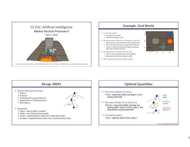
Example: ¡Grid ¡World ¡ CS ¡232: ¡Ar)ficial ¡Intelligence ¡ ¡ Markov ¡Decision ¡Processes ¡II ¡ § A ¡maze-­‑like ¡problem ¡ Oct ¡1 st , ¡2015 ¡ § The ¡agent ¡lives ¡in ¡a ¡grid ¡ Walls ¡block ¡the ¡agent’s ¡path ¡ § § Noisy ¡movement: ¡ac)ons ¡do ¡not ¡always ¡go ¡as ¡planned ¡ 80% ¡of ¡the ¡)me, ¡the ¡ac)on ¡North ¡takes ¡the ¡agent ¡North ¡ ¡ § 10% ¡of ¡the ¡)me, ¡North ¡takes ¡the ¡agent ¡West; ¡10% ¡East ¡ § If ¡there ¡is ¡a ¡wall ¡in ¡the ¡direc)on ¡the ¡agent ¡would ¡have ¡ § been ¡taken, ¡the ¡agent ¡stays ¡put ¡ § The ¡agent ¡receives ¡rewards ¡each ¡)me ¡step ¡ Small ¡“living” ¡reward ¡each ¡step ¡(can ¡be ¡nega)ve) ¡ § Big ¡rewards ¡come ¡at ¡the ¡end ¡(good ¡or ¡bad) ¡ § § Goal: ¡maximize ¡sum ¡of ¡(discounted) ¡rewards ¡ [These ¡slides ¡were ¡created ¡by ¡Dan ¡Klein ¡and ¡Pieter ¡Abbeel ¡for ¡CS188 ¡Intro ¡to ¡AI ¡at ¡UC ¡Berkeley. ¡ ¡All ¡CS188 ¡materials ¡are ¡available ¡at ¡hNp://ai.berkeley.edu.] ¡ Recap: ¡MDPs ¡ Op)mal ¡Quan))es ¡ § Markov ¡decision ¡processes: ¡ § The ¡value ¡(u)lity) ¡of ¡a ¡state ¡s: ¡ s § States ¡S ¡ V * (s) ¡= ¡expected ¡u)lity ¡star)ng ¡in ¡s ¡and ¡ s is a § Ac)ons ¡A ¡ a s ac)ng ¡op)mally ¡ state § Transi)ons ¡P(s’|s,a) ¡(or ¡T(s,a,s’)) ¡ s, ¡a ¡ a § Rewards ¡R(s,a,s’) ¡(and ¡discount ¡ γ ) ¡ (s, a) is a § The ¡value ¡(u)lity) ¡of ¡a ¡q-­‑state ¡(s,a): ¡ § Start ¡state ¡s 0 ¡ s, a q-state s,a,s ’ ¡ Q * (s,a) ¡= ¡expected ¡u)lity ¡star)ng ¡out ¡ s ’ ¡ having ¡taken ¡ac)on ¡a ¡from ¡state ¡s ¡and ¡ s,a,s’ (s,a,s’) is a § Quan))es: ¡ (thereaher) ¡ac)ng ¡op)mally ¡ transition § Policy ¡= ¡map ¡of ¡states ¡to ¡ac)ons ¡ s’ ¡ § U)lity ¡= ¡sum ¡of ¡discounted ¡rewards ¡ § The ¡op)mal ¡policy: ¡ § Values ¡= ¡expected ¡future ¡u)lity ¡from ¡a ¡state ¡(max ¡node) ¡ π * (s) ¡= ¡op)mal ¡ac)on ¡from ¡state ¡s ¡ § Q-­‑Values ¡= ¡expected ¡future ¡u)lity ¡from ¡a ¡q-­‑state ¡(chance ¡node) ¡ [Demo: ¡ ¡gridworld ¡values ¡(L9D1)] ¡ 1

Gridworld ¡Values ¡V* ¡ Gridworld: ¡Q* ¡ The ¡Bellman ¡Equa)ons ¡ The ¡Bellman ¡Equa)ons ¡ § Defini)on ¡of ¡“op)mal ¡u)lity” ¡via ¡expec)max ¡recurrence ¡ s gives ¡a ¡simple ¡one-­‑step ¡lookahead ¡rela)onship ¡ a How ¡to ¡be ¡op)mal: ¡ amongst ¡op)mal ¡u)lity ¡values ¡ ¡ s, ¡a ¡ ¡ ¡ ¡ ¡Step ¡1: ¡Take ¡correct ¡first ¡ac)on ¡ ¡ s,a,s ’ ¡ ¡ ¡ ¡ ¡Step ¡2: ¡Keep ¡being ¡op)mal ¡ s ’ ¡ § These ¡are ¡the ¡Bellman ¡equa)ons, ¡and ¡they ¡characterize ¡ op)mal ¡values ¡in ¡a ¡way ¡we’ll ¡use ¡over ¡and ¡over ¡ ¡ ¡ 2

Value ¡Itera)on ¡ Convergence* ¡ § Bellman ¡equa)ons ¡characterize ¡the ¡op)mal ¡values: ¡ § How ¡do ¡we ¡know ¡the ¡V k ¡vectors ¡are ¡going ¡to ¡converge? ¡ V(s) ¡ § Case ¡1: ¡If ¡the ¡tree ¡has ¡maximum ¡depth ¡M, ¡then ¡V M ¡holds ¡ a the ¡actual ¡untruncated ¡values ¡ s, ¡a ¡ § Case ¡2: ¡If ¡the ¡discount ¡is ¡less ¡than ¡1 ¡ s,a,s ’ ¡ § Sketch: ¡For ¡any ¡state ¡V k ¡and ¡V k+1 ¡can ¡be ¡viewed ¡as ¡depth ¡k § Value ¡itera)on ¡computes ¡them: ¡ V(s’) ¡ +1 ¡expec)max ¡results ¡in ¡nearly ¡iden)cal ¡search ¡trees ¡ § The ¡difference ¡is ¡that ¡on ¡the ¡boNom ¡layer, ¡V k+1 ¡has ¡actual ¡ rewards ¡while ¡V k ¡has ¡zeros ¡ § That ¡last ¡layer ¡is ¡at ¡best ¡all ¡R MAX ¡ ¡ § It ¡is ¡at ¡worst ¡R MIN ¡ ¡ § But ¡everything ¡is ¡discounted ¡by ¡γ k ¡that ¡far ¡out ¡ § Value ¡itera)on ¡is ¡just ¡a ¡fixed ¡point ¡solu)on ¡method ¡ § So ¡V k ¡and ¡V k+1 ¡are ¡at ¡most ¡γ k ¡max|R| ¡different ¡ § … ¡though ¡the ¡V k ¡vectors ¡are ¡also ¡interpretable ¡as ¡)me-­‑limited ¡values ¡ § So ¡as ¡k ¡increases, ¡the ¡values ¡converge ¡ Policy ¡Methods ¡ Policy ¡Evalua)on ¡ 3

Fixed ¡Policies ¡ U)li)es ¡for ¡a ¡Fixed ¡Policy ¡ Do ¡the ¡op)mal ¡ac)on ¡ Do ¡what ¡ π ¡says ¡to ¡do ¡ § Another ¡basic ¡opera)on: ¡compute ¡the ¡u)lity ¡of ¡a ¡state ¡s ¡ s under ¡a ¡fixed ¡(generally ¡non-­‑op)mal) ¡policy ¡ s s π (s) ¡ a π (s) ¡ § Define ¡the ¡u)lity ¡of ¡a ¡state ¡s, ¡under ¡a ¡fixed ¡policy ¡ π : ¡ s, ¡ π (s) ¡ s, ¡a ¡ s, ¡ π (s) ¡ V π (s) ¡= ¡expected ¡total ¡discounted ¡rewards ¡star)ng ¡in ¡s ¡and ¡following ¡ π ¡ s, ¡ π (s),s ’ ¡ s,a,s ’ ¡ s, ¡ π (s),s ’ ¡ s ’ ¡ § Recursive ¡rela)on ¡(one-­‑step ¡look-­‑ahead ¡/ ¡Bellman ¡equa)on): ¡ s ’ ¡ s ’ ¡ § Expec)max ¡trees ¡max ¡over ¡all ¡ac)ons ¡to ¡compute ¡the ¡op)mal ¡values ¡ § If ¡we ¡fixed ¡some ¡policy ¡ π (s), ¡then ¡the ¡tree ¡would ¡be ¡simpler ¡– ¡only ¡one ¡ac)on ¡per ¡state ¡ § … ¡though ¡the ¡tree’s ¡value ¡would ¡depend ¡on ¡which ¡policy ¡we ¡fixed ¡ Example: ¡Policy ¡Evalua)on ¡ Example: ¡Policy ¡Evalua)on ¡ Always ¡Go ¡Right ¡ Always ¡Go ¡Forward ¡ Always ¡Go ¡Right ¡ Always ¡Go ¡Forward ¡ 4

Policy ¡Evalua)on ¡ Policy ¡Extrac)on ¡ § How ¡do ¡we ¡calculate ¡the ¡V’s ¡for ¡a ¡fixed ¡policy ¡ π ? ¡ s π (s) ¡ § Idea ¡1: ¡Turn ¡recursive ¡Bellman ¡equa)ons ¡into ¡updates ¡ ¡(like ¡value ¡itera)on) ¡ s, ¡ π (s) ¡ s, ¡ π (s),s ’ ¡ s ’ ¡ § Efficiency: ¡O(S 2 ) ¡per ¡itera)on ¡ § Idea ¡2: ¡Without ¡the ¡maxes, ¡the ¡Bellman ¡equa)ons ¡are ¡just ¡a ¡linear ¡system ¡ § Solve ¡with ¡Matlab ¡(or ¡your ¡favorite ¡linear ¡system ¡solver) ¡ Compu)ng ¡Ac)ons ¡from ¡Values ¡ Compu)ng ¡Ac)ons ¡from ¡Q-­‑Values ¡ § Let’s ¡imagine ¡we ¡have ¡the ¡op)mal ¡values ¡V*(s) ¡ § Let’s ¡imagine ¡we ¡have ¡the ¡op)mal ¡q-­‑values: ¡ § How ¡should ¡we ¡act? ¡ § How ¡should ¡we ¡act? ¡ § It’s ¡not ¡obvious! ¡ § Completely ¡trivial ¡to ¡decide! ¡ § We ¡need ¡to ¡do ¡a ¡mini-­‑expec)max ¡(one ¡step) ¡ § This ¡is ¡called ¡policy ¡extrac)on, ¡since ¡it ¡gets ¡the ¡policy ¡implied ¡by ¡the ¡values ¡ § Important ¡lesson: ¡ac)ons ¡are ¡easier ¡to ¡select ¡from ¡q-­‑values ¡than ¡values! ¡ 5

Policy ¡Itera)on ¡ Problems ¡with ¡Value ¡Itera)on ¡ § Value ¡itera)on ¡repeats ¡the ¡Bellman ¡updates: ¡ s a s, ¡a ¡ s,a,s ’ ¡ § Problem ¡1: ¡It’s ¡slow ¡– ¡O(S 2 A) ¡per ¡itera)on ¡ s ’ ¡ § Problem ¡2: ¡The ¡“max” ¡at ¡each ¡state ¡rarely ¡changes ¡ § Problem ¡3: ¡The ¡policy ¡ohen ¡converges ¡long ¡before ¡the ¡values ¡ [Demo: ¡value ¡itera)on ¡(L9D2)] ¡ k=0 ¡ k=1 ¡ Noise ¡= ¡0.2 ¡ Noise ¡= ¡0.2 ¡ Discount ¡= ¡0.9 ¡ Discount ¡= ¡0.9 ¡ Living ¡reward ¡= ¡0 ¡ Living ¡reward ¡= ¡0 ¡ 6

k=2 ¡ k=3 ¡ Noise ¡= ¡0.2 ¡ Noise ¡= ¡0.2 ¡ Discount ¡= ¡0.9 ¡ Discount ¡= ¡0.9 ¡ Living ¡reward ¡= ¡0 ¡ Living ¡reward ¡= ¡0 ¡ k=4 ¡ k=5 ¡ Noise ¡= ¡0.2 ¡ Noise ¡= ¡0.2 ¡ Discount ¡= ¡0.9 ¡ Discount ¡= ¡0.9 ¡ Living ¡reward ¡= ¡0 ¡ Living ¡reward ¡= ¡0 ¡ 7

k=6 ¡ k=7 ¡ Noise ¡= ¡0.2 ¡ Noise ¡= ¡0.2 ¡ Discount ¡= ¡0.9 ¡ Discount ¡= ¡0.9 ¡ Living ¡reward ¡= ¡0 ¡ Living ¡reward ¡= ¡0 ¡ k=8 ¡ k=9 ¡ Noise ¡= ¡0.2 ¡ Noise ¡= ¡0.2 ¡ Discount ¡= ¡0.9 ¡ Discount ¡= ¡0.9 ¡ Living ¡reward ¡= ¡0 ¡ Living ¡reward ¡= ¡0 ¡ 8