recap lexicalized pcfgs
play

Recap: Lexicalized PCFGs We now need to estimate rule probabilities - PowerPoint PPT Presentation

Recap: Lexicalized PCFGs We now need to estimate rule probabilities such as Prob ( S(questioned,Vt) NP(lawyer,NN) VP(questioned,Vt) | S(questioned,Vt) ) 6.864 (Fall 2007): Lecture 5 Sparse data is a problem. We have a huge number of


  1. Recap: Lexicalized PCFGs • We now need to estimate rule probabilities such as Prob ( S(questioned,Vt) ⇒ NP(lawyer,NN) VP(questioned,Vt) | S(questioned,Vt) ) 6.864 (Fall 2007): Lecture 5 • Sparse data is a problem. We have a huge number of non- Parsing and Syntax III terminals, and a huge number of possible rules. We have to work hard to estimate these rule probabilities... • Once we have estimated these rule probabilities, we can find the highest scoring parse tree under the lexicalized PCFG using dynamic programming methods (see Problem set 1). 1 3 
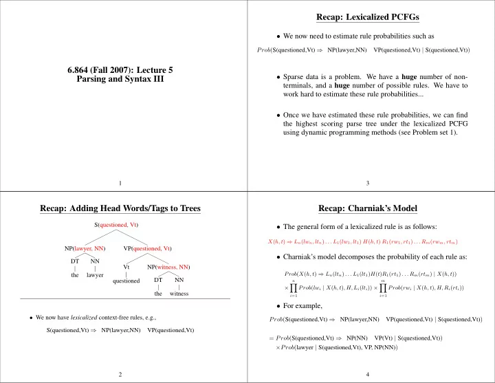
Recap: Adding Head Words/Tags to Trees Recap: Charniak’s Model S(questioned, Vt) • The general form of a lexicalized rule is as follows: X ( h, t ) ⇒ L n ( lw n , lt n ) . . . L 1 ( lw 1 , lt 1 ) H ( h, t ) R 1 ( rw 1 , rt 1 ) . . . R m ( rw m , rt m ) NP(lawyer, NN) VP(questioned, Vt) • Charniak’s model decomposes the probability of each rule as: DT NN Vt NP(witness, NN) Prob ( X ( h, t ) ⇒ L n ( lt n ) . . . L 1 ( lt 1 ) H ( t ) R 1 ( rt 1 ) . . . R m ( rt m ) | X ( h, t )) the lawyer DT NN questioned n m � � × Prob ( lw i | X ( h, t ) , H, L i ( lt i )) × Prob ( rw i | X ( h, t ) , H, R i ( rt i )) the witness i =1 i =1 • For example, • We now have lexicalized context-free rules, e.g., Prob ( S(questioned,Vt) ⇒ NP(lawyer,NN) VP(questioned,Vt) | S(questioned,Vt) ) S(questioned,Vt) ⇒ NP(lawyer,NN) VP(questioned,Vt) = Prob ( S(questioned,Vt) ⇒ NP(NN) VP(Vt) | S(questioned,Vt) ) = × Prob ( lawyer | S(questioned,Vt), VP, NP(NN) ) 2 4

  2. Motivation for Breaking Down Rules The General Form of Model 1 • The general form of a lexicalized rule is as follows: • First step of decomposition of (Charniak 1997): S(questioned,Vt) X ( h, t ) ⇒ L n ( lw n , lt n ) . . . L 1 ( lw 1 , lt 1 ) H ( h, t ) R 1 ( rw 1 , rt 1 ) . . . R m ( rw m , rt m ) ⇓ P ( NP(NN) VP | S(questioned,Vt) ) • Collins model 1 decomposes the probability of each rule as: S(questioned,Vt) P h ( H | X, h, t ) × NP( ,NN) VP(questioned,Vt) n � P d ( L i ( lw i , lt i ) | X, H, h, t, LEFT ) × i =1 • Relies on counts of entire rules P d ( STOP | X, H, h, t, LEFT ) × • These counts are sparse : m � P d ( R i ( rw i , rt i ) | X, H, h, t, RIGHT ) × i =1 – 40,000 sentences from Penn treebank have 12,409 rules. P d ( STOP | X, H, h, t, RIGHT ) – 15% of all test data sentences contain a rule never seen in training 5 7 Modeling Rule Productions as Markov Processes • P h term is a head-label probability • Collins (1997), Model 1 • P d terms are dependency probabilities • Both the P h and P d terms are smoothed, using similar S(told,V) techniques to Charniak’s model STOP NP(yesterday,NN) NP(Hillary,NNP) VP(told,V) STOP We first generate the head label of the rule Then generate the left modifiers Then generate the right modifiers P h ( VP | S, told, V ) × P d ( NP(Hillary,NNP) | S,VP,told,V,LEFT ) × P d ( NP(yesterday,NN) | S,VP,told,V,LEFT ) × P d ( STOP | S,VP,told,V,LEFT ) × P d ( STOP | S,VP,told,V,RIGHT ) 6 8

  3. Overview of Today’s Lecture A Refi nement: Adding a Distance Variable • Refinements to Model 1 • ∆ = 1 if position is adjacent to the head. • Evaluating parsing models S(told,V) • Extensions to the parsing models ?? NP(Hillary,NNP) VP(told,V) ⇓ S(told,V) NP(yesterday,NN) NP(Hillary,NNP) VP(told,V) P h ( VP | S, told, V ) × P d ( NP(Hillary,NNP) | S,VP,told,V,LEFT ) × P d ( NP(yesterday,NN) | S,VP,told,V,LEFT, ∆ = 0) 9 11 A Refi nement: Adding a Distance Variable The Final Probabilities S(told,V) • ∆ = 1 if position is adjacent to the head, 0 otherwise S(told,V) STOP NP(yesterday,NN) NP(Hillary,NNP) VP(told,V) STOP ?? VP(told,V) P h ( VP | S, told, V ) × P d ( NP(Hillary,NNP) | S,VP,told,V,LEFT, ∆ = 1) × ⇓ P d ( NP(yesterday,NN) | S,VP,told,V,LEFT, ∆ = 0) × P d ( STOP | S,VP,told,V,LEFT, ∆ = 0) × S(told,V) P d ( STOP | S,VP,told,V,RIGHT, ∆ = 1) NP(Hillary,NNP) VP(told,V) P h ( VP | S, told, V ) × P d ( NP(Hillary,NNP) | S,VP,told,V,LEFT, ∆ = 1) 10 12

  4. Adding the Complement/Adjunct Distinction Complements vs. Adjuncts S • Complements are closely related to the head they modify, NP VP adjuncts are more indirectly related • Complements are usually arguments of the thing they modify S(told,V) subject V yesterday Hillary told . . . ⇒ Hillary is doing the telling verb • Adjuncts add modifying information: time, place, manner etc. yesterday Hillary told . . . ⇒ yesterday is a temporal modifier NP(yesterday,NN) NP(Hillary,NNP) VP(told,V) • Complements are usually required, adjuncts are optional V . . . NN NNP told yesterday Hillary vs. yesterday Hillary told . . . (grammatical) vs. Hillary told . . . (grammatical) • Hillary is the subject vs. yesterday told . . . (ungrammatical) • yesterday is a temporal modifier • But nothing to distinguish them. 13 15 Adding the Complement/Adjunct Distinction Adding Tags Making the Complement/Adjunct Distinction VP S S V NP NP-C VP NP VP VP(told,V) verb object subject V modifier V verb verb V NP(Bill,NNP) NP(yesterday,NN) SBAR(that,COMP) S(told,V) told NNP NN . . . Bill yesterday NP(yesterday,NN) NP-C(Hillary,NNP) VP(told,V) • Bill is the object . . . V NN NNP • yesterday is a temporal modifier told yesterday Hillary • But nothing to distinguish them. 14 16

  5. Adding Tags Making the Complement/Adjunct Distinction Adding Subcategorization Probabilities VP VP • Step 2: choose left subcategorization frame V NP-C V NP verb object verb modifier S(told,V) VP(told,V) VP(told,V) ⇓ V NP-C(Bill,NNP) NP(yesterday,NN) SBAR-C(that,COMP) S(told,V) told NNP NN . . . VP(told,V) Bill yesterday { NP-C } P h ( VP | S, told, V ) × P lc ( { NP-C } | S, VP, told, V ) 17 19 Adding Subcategorization Probabilities • Step 3: generate left modifiers in a Markov chain • Step 1: generate category of head child S(told,V) ?? VP(told,V) S(told,V) { NP-C } ⇓ ⇓ S(told,V) S(told,V) VP(told,V) NP-C(Hillary,NNP) VP(told,V) {} P h ( VP | S, told, V ) P h ( VP | S, told, V ) × P lc ( { NP-C } | S, VP, told, V ) × P d ( NP-C(Hillary,NNP) | S,VP,told,V,LEFT, { NP-C } ) 18 20

  6. The Final Probabilities S(told,V) S(told,V) ?? NP-C(Hillary,NNP) VP(told,V) STOP NP(yesterday,NN) NP-C(Hillary,NNP) VP(told,V) STOP {} ⇓ P h ( VP | S, told, V ) × S(told,V) P lc ( { NP-C } | S, VP, told, V ) × P d ( NP-C(Hillary,NNP) | S,VP,told,V,LEFT, ∆ = 1 , { NP-C } ) × P d ( NP(yesterday,NN) | S,VP,told,V,LEFT, ∆ = 0 , {} ) × P d ( STOP | S,VP,told,V,LEFT, ∆ = 0 , {} ) × P rc ( {} | S, VP, told, V ) × NP(yesterday,NN) NP-C(Hillary,NNP) VP(told,V) {} P d ( STOP | S,VP,told,V,RIGHT, ∆ = 1 , {} ) P h ( VP | S, told, V ) × P lc ( { NP-C } | S, VP, told, V ) P d ( NP-C(Hillary,NNP) | S,VP,told,V,LEFT, { NP-C } ) × P d ( NP(yesterday,NN) | S,VP,told,V,LEFT, {} ) 21 23 Another Example S(told,V) VP(told,V) ?? NP(yesterday,NN) NP-C(Hillary,NNP) VP(told,V) {} ⇓ V(told,V) NP-C(Bill,NNP) NP(yesterday,NN) SBAR-C(that,COMP) S(told,V) P h ( V | VP, told, V ) × P lc ( {} | VP, V, told, V ) × P d ( STOP | VP,V,told,V,LEFT, ∆ = 1 , {} ) × P rc ( { NP-C, SBAR-C } | VP, V, told, V ) × STOP NP(yesterday,NN) NP-C(Hillary,NNP) VP(told,V) P d ( NP-C(Bill,NNP) | VP,V,told,V,RIGHT, ∆ = 1 , { NP-C, SBAR-C } ) × {} P d ( NP(yesterday,NN) | VP,V,told,V,RIGHT, ∆ = 0 , { SBAR-C } ) × P d ( SBAR-C(that,COMP) | VP,V,told,V,RIGHT, ∆ = 0 , { SBAR-C } ) × P h ( VP | S, told, V ) × P lc ( { NP-C } | S, VP, told, V ) P d ( STOP | VP,V,told,V,RIGHT, ∆ = 0 , {} ) P d ( NP-C(Hillary,NNP) | S,VP,told,V,LEFT, { NP-C } ) × P d ( NP(yesterday,NN) | S,VP,told,V,LEFT, {} ) × P d ( STOP | S,VP,told,V,LEFT, {} ) 22 24

  7. Summary Evaluation: Representing Trees as Constituents S • Identify heads of rules ⇒ dependency representations NP VP • Presented two variants of PCFG methods applied to DT NN lexicalized grammars . Vt NP the lawyer DT NN – Break generation of rule down into small (markov questioned process) steps the witness – Build dependencies back up (distance, subcategorization) ⇓ Label Start Point End Point NP 1 2 NP 4 5 VP 3 5 S 1 5 25 27 Overview of Today’s Lecture Precision and Recall Label Start Point End Point • Refinements to Model 1 Label Start Point End Point NP 1 2 NP 1 2 • Evaluating parsing models NP 4 5 NP 4 5 NP 4 8 PP 6 8 PP 6 8 • Extensions to the parsing models NP 7 8 NP 7 8 VP 3 8 VP 3 8 S 1 8 S 1 8 • G = number of constituents in gold standard = 7 • P = number in parse output = 6 • C = number correct = 6 Recall = 100% × C G = 100% × 6 Precision = 100% × C P = 100% × 6 7 6 26 28

Download Presentation
Download Policy: The content available on the website is offered to you 'AS IS' for your personal information and use only. It cannot be commercialized, licensed, or distributed on other websites without prior consent from the author. To download a presentation, simply click this link. If you encounter any difficulties during the download process, it's possible that the publisher has removed the file from their server.

Recommend


More recommend