
SLIDE 1
Re-indexing the DFT (n and k)
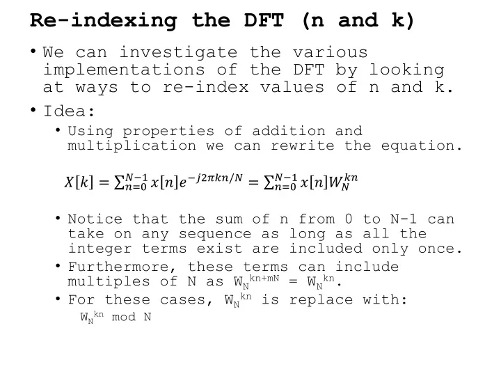
- We can investigate the various
implementations of the DFT by looking at ways to re-index values of n and k.
- Idea:
- Using properties of addition and
multiplication we can rewrite the equation. 𝑌 𝑙 = σ𝑜=0
𝑂−1 𝑦 𝑜 𝑓−𝑘2𝜌𝑙𝑜/𝑂 = σ𝑜=0 𝑂−1 𝑦 𝑜 𝑋 𝑂 𝑙𝑜
- Notice that the sum of n from 0 to N-1 can
take on any sequence as long as all the integer terms exist are included only once.
- Furthermore, these terms can include
multiples of N as WN
kn+mN = WN kn.
- For these cases, WN
kn is replace with:
WN
kn mod N