!1
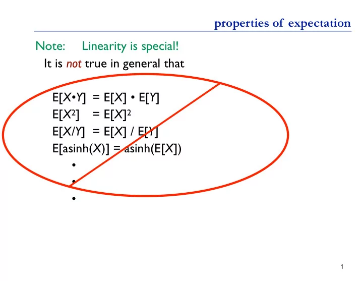
properties of expectation Note: Linearity is special! It is not true in general that E[X•Y] = E[X] • E[Y] E[X2] = E[X]2 E[X/Y] = E[X] / E[Y] E[asinh(X)] = asinh(E[X])

properties of expectation Note: Linearity is special! It is not - - PowerPoint PPT Presentation
properties of expectation Note: Linearity is special! It is not true in general that E[ XY ] = E[ X ] E[ Y ] E[ X 2 ] = E[ X ] 2 E[ X/Y ] = E[ X ] / E[ Y ] E[asinh( X )] = asinh(E[ X ]) ! 1 variance E Cx X ENDY EAT Van
!1
properties of expectation Note: Linearity is special! It is not true in general that E[X•Y] = E[X] • E[Y] E[X2] = E[X]2 E[X/Y] = E[X] / E[Y] E[asinh(X)] = asinh(E[X])
!2
Van x
E
X ENDY
X
standarddeviation
a2Var X
a b
are constants
more variance examples
!3
2 4 0.00 0.10
2 4 0.00 0.10
2 4 0.00 0.10
2 4 0.00 0.10 0.20
σ2 = 5.83 σ2 = 10 σ2 = 15 σ2 = 19.7
p
Pr Xix
X
!4
Van
Van XH
Van X
Van Y
in general
ExampleI
Ea
I
Y
X
F
Y
Vanly
L Van
Vav
2
Van XH
O Exa
Van
Xix
Van
2X
2 Van
4 Vana
Vallytvalx
!5
Random variables
independence Arau
X and
an event E are independent f
Fx Pr X
x
NE
Pr X
x PrlE
2r.vn's X
Y
are independent
Kitty
Pr X xnY y
PrfX x PrCY y
Flip
in
independently 2h times
Zn
heads in 2h tresses
Xi
heads
in
Austin
tosses
ya
He heads
in 2nd n
tosses X
Y indep
X
Z notindep
pr x i
find 7
I
prfx.u.az
fPrfX
x Prl2
j
lngn1
t.FM
O
Zen
Prix.im j
7 j Lat
2h
!6
Thmi
X
Y
are independent
then E XuY
E X E Y
F XY
ab
Pr n'Kb
a b Prcx
a
Prats
bgk.LK
aPrCX
a
bPrCY
b
I
EH
EG
Z
I
2
4
2
7
9
Theorem: If X & Y are independent, then Var[X+Y] = Var[X]+Var[Y] Proof: variance of independent r.v.s is additive
!10
!11
discrete uniform random variables A discrete random variable X equally likely to take any (integer) value between integers a and b, inclusive, is uniform. Notation: Probability mass function: Mean: Variance:
!12
Toss die
1,2 as
a
at
at2
a b
9 1
b 6
b
it'ra b3
Pr X
i
are
2
b a
b at2
12
discrete uniform random variables A discrete random variable X equally likely to take any (integer) value between integers a and b, inclusive, is uniform. Notation: X ~ Unif(a,b) Probability: Mean, Variance: Example: value shown on one roll of a fair die is Unif(1,6): P(X=i) = 1/6 E[X] = 7/2 Var[X] = 35/12
!13
1 2 3 4 5 6 7 0.10 0.16 0.22 i P(X=i)
In a series X1, X2, ... of Bernoulli trials with success probability p, let Y be the index of the first success, i.e., X1 = X2 = ... = XY-1 = 0 & XY = 1 Then Y is a geometric random variable with parameter p.
Examples: Number of coin flips until first head Number of blind guesses on SAT until I get one right Number of darts thrown until you hit a bullseye Number of random probes into hash table until empty slot Number of wild guesses at a password until you hit it
Probability mass function: Mean: Variance: geometric distribution
!14
cointosses with P
upht
X
n GeoCp
TT
Chp4p
i
Ip
i
p
pr X
L
p2
In a series X1, X2, ... of Bernoulli trials with success probability p, let Y be the index of the first success, i.e., X1 = X2 = ... = XY-1 = 0 & XY = 1 Then Y is a geometric random variable with parameter p.
Examples: Number of coin flips until first head Number of blind guesses on SAT until I get one right Number of darts thrown until you hit a bullseye Number of random probes into hash table until empty slot Number of wild guesses at a password until you hit it
P(Y=k) = (1-p)k-1p; Mean 1/p; Variance (1-p)/p2 geometric distribution
!15
Bernoulli random variables An experiment results in “Success” or “Failure” X is an indicator random variable (1 = success, 0 = failure) P(X=1) = p and P(X=0) = 1-p X is called a Bernoulli random variable: X ~ Ber(p) Mean: Variance:
!16
indicator
riv
4 II
expectation s I
p
O
O l p
E
p tp
xeRangelx
Vancx
E XY
Efx
2
p
Bernoulli random variables An experiment results in “Success” or “Failure” X is an indicator random variable (1 = success, 0 = failure) P(X=1) = p and P(X=0) = 1-p X is called a Bernoulli random variable: X ~ Ber(p) E[X] = E[X2] = p Var(X) = E[X2] – (E[X])2 = p – p2 = p(1-p) Examples: coin flip random binary digit whether a disk drive crashed
!17 Jacob (aka James, Jacques) Bernoulli, 1654 – 1705