Program 2 Corrections/Clarifications CPSC 314 Computer Graphics - PDF document

University of British Columbia Program 2 Corrections/Clarifications CPSC 314 Computer Graphics � handin 314 proj2 (not 414) Jan-Apr 2005 � ‘f’ not ‘s’ to toggle flat/smooth shading Tamara Munzner � ‘s’ already in use for camera � add: ‘t’ to toggle between randomly colored and Prog 2, Kangaroo Hall of Fame, grey terrain Midterm Review, � makes it easier to check if lighting correct (Interpolation if time) � add: ‘u’ to replace terrain with new randomly Week 6, Wed Feb 9 generated geometry � consider adding for a bit of extra credit: http://www.ugrad.cs.ubc.ca/~cs314/Vjan2005 � ‘+/-’ toggle to increment/decrement abs cam speed 2 Program 2 Corrections/Clarifications Program 2 Quick Demo � 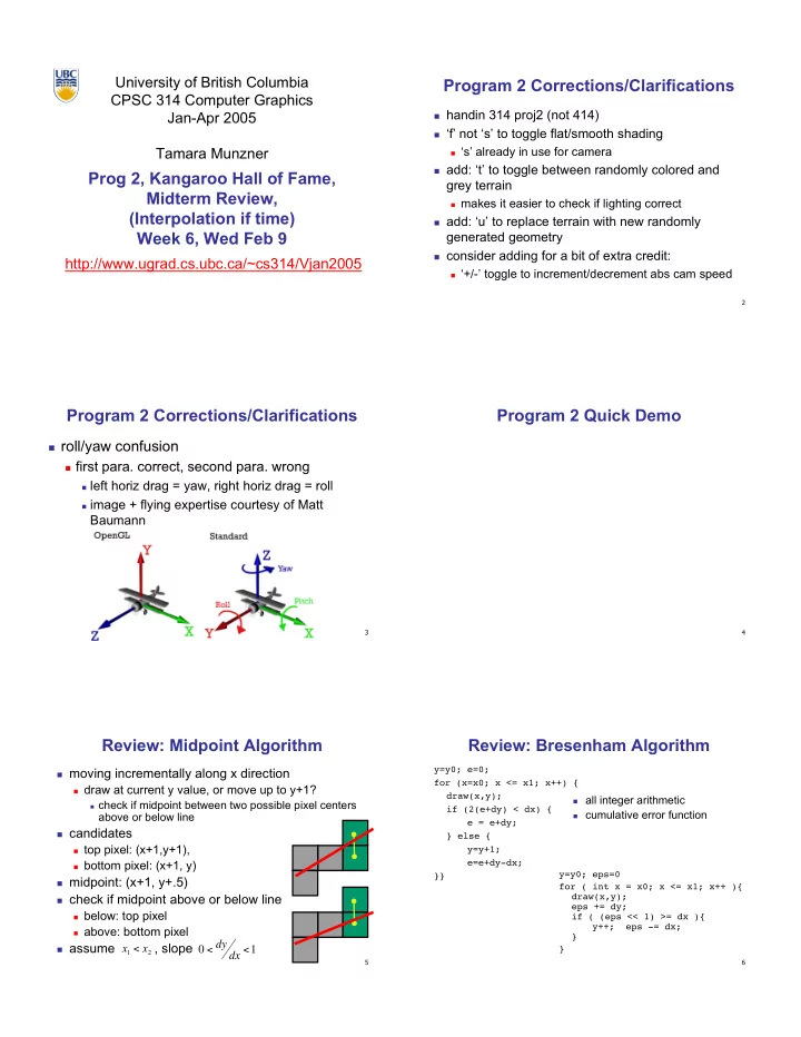roll/yaw confusion � first para. correct, second para. wrong � left horiz drag = yaw, right horiz drag = roll � image + flying expertise courtesy of Matt Baumann 3 4 Review: Midpoint Algorithm Review: Bresenham Algorithm y=y0; e=0; � moving incrementally along x direction for (x=x0; x <= x1; x++) { � draw at current y value, or move up to y+1? draw(x,y); � all integer arithmetic � check if midpoint between two possible pixel centers if (2(e+dy) < dx) { � cumulative error function above or below line e = e+dy; � candidates } else { � top pixel: (x+1,y+1), y=y+1; e=e+dy-dx; � bottom pixel: (x+1, y) y=y0; eps=0 }} � midpoint: (x+1, y+.5) for ( int x = x0; x <= x1; x++ ){ � check if midpoint above or below line draw(x,y); eps += dy; � below: top pixel if ( (eps << 1) >= dx ){ y++; eps -= dx; � above: bottom pixel } 0 < dy � assume , slope x < x dx < 1 } 1 2 5 6

Review: Flood Fill Review: Scanline Algorithms � draw polygon edges, seed point, recursively � set pixels inside polygon boundary along set all neighbors until boundary is hit to fill horizontal lines one pixel apart interior � drawbacks: visit pixels up to 4x, per-pixel � use bounding box to speed up memory storage needed P 3 1 5=0 2 P 4 7 Review: Edge Walking Review: General Polygon Rasterization � basic idea: � draw edges vertically � interpolate colors down edges � idea: use a parity test � fill in horizontal spans for each for each scanline scanline edgeCnt = 0; � at each scanline, interpolate for each pixel on scanline (l to r) edge colors across span if (oldpixel->newpixel crosses edge) edgeCnt ++; // draw the pixel if edgeCnt odd if (edgeCnt % 2) setPixel(pixel); 9 10 But Wait, There’s More! � nice comment :) � “this project is fun, only one of the very few that I actually enjoyed. Too bad there's only one CG course in UBC =( Hall of Fame � two fourth year CG courses await you! � 424 Geometric Modelling � 426 Animation 11 12

Midterm Exam � Friday Feb 11 10am-10:50am � you may use one handwritten 8.5”x11” sheet � one side of page � no other notes, no books Midterm Review � nonprogrammable calculators OK � arrive on time! � sit every other seat, ID out in front of you � coats and bags in front of room 13 14 What’s Covered Reading � transformations � FCS book, Red book � viewing and projections � see web page for details � you can be tested on material in book but not � coordinate systems of rendering pipeline covered in lecture � lighting and shading � you can be tested on material covered in lecture but not covered in book � not scan conversion 15 16 Old Exams Posted The Rendering Pipeline � see course web page � pros and cons of pipeline approach Model/View Model/View Geometry Geometry Model/View Perspective Perspective Perspective Geometry Lighting Lighting Lighting Clipping Clipping Clipping Transform. Transform. Transform. Transform. Database Database Database Transform. Transform. Frame- Frame- Scan Scan Depth Depth Frame- Scan Depth Texturing Texturing Texturing Blending Blending Blending buffer Conversion buffer buffer Conversion Conversion Test Test Test 17 18

Transformations Homogeneous Coordinates � x w x w � � � � � � � � � � translate(a,b,c) translate(a,b,c) scale(a,b,c) scale(a,b,c) y w y w w w � � � � � � x ' 1 a x x ' a x � � � � � � w w � � � � � � � � � � � � � � � � � � � � � � � � � � y ' 1 b y y ' b y � � � � � � � � � � � � = = z ' c z z ' 1 c z � � � � � � � � � � � � � � � � � � � � � � � � 1 1 1 1 1 1 � � � � � � x � � � � � � x � � � � w= 1 w= 1 � � � � y y Rotate ( x , ) Rotate ( y , ) Rotate ( z , ) � � � � � � � 1 � 1 � � � � � x ' 1 x cos sin cos sin � � � � � � � � � � � � � � � � � � � � � � � � � � � y ' cos sin y 1 sin cos � � � � � � � � � � � � � � � = y y 1 � z ' � � sin cos � � z � sin cos � � � � � � � � � � � � � � � � � � � 1 1 1 1 1 � � � � � � � � � � x x 19 20 Composing Transformations Composing Transformations � example: rotation around arbitrary center Ta Tb = Tb Ta, but Ra Rb Rb != != Rb Rb Ra and Ta Ra and Ta Rb Rb != != Rb Rb Ta Ta Ta Tb = Tb Ta, but Ra 21 22 Composing Transformations Composing Transformations � example: rotation around arbitrary center � example: rotation around arbitrary center � step 1: translate coordinate system to rotation � step 2: perform rotation center 23 24

Composing Transformations Composing Transformations � example: rotation around arbitrary center � rotation about a fixed point � step 3: back to original coordinate system p’ = TRT -1 p � rotation around an arbitrary axis OpenGL: � considering frame vs. object D � p’ = DCBAp C frame B A draw p object 25 26 Matrix Stacks Transformation Hierarchies � hierarchies don’t fall apart when changed � push and pop matrix stack � transforms apply to graph nodes beneath � avoid computing inverses or incremental xforms � avoid numerical error T T 2 2 (x) (x) T 1 (x) T 1 (x) T 3 (x) T 3 (x) World coordinates World coordinates 27 28 Matrix Stacks Transformation Hierarchies � example glTranslate3f(x,y,0); glTranslate3f(x,y,0); glRotatef( ,0,0,1); ( ,0,0,1); glRotatef � D = C scale(2,2,2) trans(1,0,0) D = C scale(2,2,2) trans(1,0,0) 1 glPushMatrix glPushMatrix() () DrawBody DrawBody(); (); glPushMatrix(); (); glPushMatrix glPopMatrix() glPopMatrix () � glTranslate3f(0,7,0); glTranslate3f(0,7,0); 2 C C D D � DrawHead(); (); DrawHead DrawSquare() DrawSquare () 4 glPopMatrix(); glPopMatrix (); C C C C C glPushMatrix() () C C C glPushMatrix glPushMatrix(); (); glPushMatrix glScale3f(2,2,2) glScale3f(2,2,2) glTranslate(2.5,5.5,0); glTranslate (2.5,5.5,0); B B B B B B B B � � glRotatef( ,0,0,1); ( ,0,0,1); glRotatef � � 3 glTranslate3f(1,0,0) glTranslate3f(1,0,0) 5 2 1 DrawUArm DrawUArm(); (); A A A A A A A A DrawSquare() DrawSquare () glTranslate(0,-3.5,0); (0,-3.5,0); glTranslate y y glPopMatrix() glPopMatrix () glRotatef glRotatef( ,0,0,1); ( ,0,0,1); � 3 DrawLArm(); (); DrawLArm x x glPopMatrix(); glPopMatrix (); ... (draw other arm) ... (draw other arm) 29 30