Produo primria - - Tpicos Tpicos Produo primria Tipos de - - PowerPoint PPT Presentation

produ o prim ria t picos t picos produ o prim ria
SMART_READER_LITE
LIVE PREVIEW

Produo primria - - Tpicos Tpicos Produo primria Tipos de - - PowerPoint PPT Presentation

Produo primria - - Tpicos Tpicos Produo primria Tipos de produtores e taxas de produo Tipos de produtores e taxas de produo Medio da produo primria Medio da produo primria


slide-1
SLIDE 1

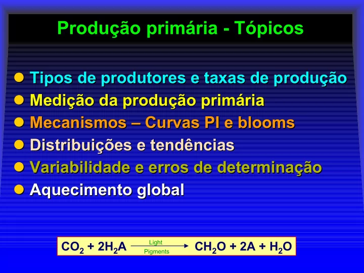
Produção primária Produção primária -

  • Tópicos

Tópicos

  • Tipos de produtores e taxas de produção

Tipos de produtores e taxas de produção

  • Medição da produção primária

Medição da produção primária

  • Mecanismos

Mecanismos – – Curvas PI e blooms Curvas PI e blooms

  • Distribuições e tendências

Distribuições e tendências

  • Variabilidade e erros de determinação

Variabilidade e erros de determinação

  • Aquecimento global

Aquecimento global

CO2 + 2H2A CH2O + 2A + H2O

Light Pigments

slide-2
SLIDE 2

Tipos de produtores Tipos de produtores

Produtor Produtor Nutrientes Nutrientes Exemplos Exemplos Fitoplâncton Fitoplâncton Coluna de água Coluna de água Diatomáceas Diatomáceas Microfitobentos Microfitobentos Coluna de água Coluna de água Diatomáceas Diatomáceas Macroalgas (algas macrófitas) Macroalgas (algas macrófitas) Coluna de água Coluna de água Fucus Fucus Vegetação de sapal Vegetação de sapal Sedimento Sedimento Spartina Spartina Angiospérmicas (“seagrasses”) Angiospérmicas (“seagrasses”) Sedimento e/ou água Sedimento e/ou água Zostera Zostera

  • Oceano aberto, águas costeiras e estuários

Oceano aberto, águas costeiras e estuários

  • Unicelulares

Unicelulares

  • Razão P/B elevada (>50)

Razão P/B elevada (>50)

  • Zonas pouco profundas (Z

Zonas pouco profundas (Zf

f > Z) ou intertidais

> Z) ou intertidais

  • Multicelulares

Multicelulares

  • Razão P/B baixa

Razão P/B baixa

slide-3
SLIDE 3

Relevância Relevância à à escala escala do do ecossistema ecossistema II II

Clorofila a (mg m-3)

Distribuição global de clorofila Distribuição global de clorofila a a estimada a estimada a partir de dados de satélite partir de dados de satélite

Dados do SEAWIFS, Verão no Hemisfério Norte (1998 Dados do SEAWIFS, Verão no Hemisfério Norte (1998-

  • 2001)

2001)

  • Prod. primária (fitoplâncton) 200-360 X 1014 gC ano-1 (98.9%)
slide-4
SLIDE 4

Diatoms Diatoms Dinoflagellates Coccoliths

Phytoplankton Phytoplankton some examples some examples

slide-5
SLIDE 5

Phytoplankton Phytoplankton -

  • diatoms

diatoms Nitschia bicapitata Nitschia bicapitata

5 5µ µm m

Chavez Chavez et al et al., 1991 ., 1991 -

  • Limnol
  • Limnol. &

. & Oceanog

  • Oceanog. 36, p. 1816

. 36, p. 1816-

  • 33

33

slide-6
SLIDE 6

SeaWifs SeaWifs image images s of

  • f

cocollith cocollith blooms blooms

Cornwall, U.K. Cornwall, U.K. Tasmania Tasmania

slide-7
SLIDE 7

Relevância para a gestão I Relevância para a gestão I “Bloom” de “Bloom” de Noctiluca Noctiluca – – California, E.U.A. California, E.U.A.

Foto cortesia de P.J.S. Franks, WHOI

slide-8
SLIDE 8

Cyanobacteria bloom Cyanobacteria bloom – – Potomac estuary Potomac estuary

This dense bloom of cyanobacteria (blue-green algae) occurred in the Potomac River estuary downstream of Washington, D.C. Photo courtesy of W. Bennett USGS.

slide-9
SLIDE 9

Em Florida Bay, este “bloom” de macroalgas colmatou as fanerogâmicas marinhas, provocando o desaparecimento desta vegetação. Foto cortesia de Brian Lapointe, Harbor Branch Oceanographic Institute.

Relevância para Relevância para a a gestão gestão III III “Bloom” de “Bloom” de macroalgas na macroalgas na Florida Florida

slide-10
SLIDE 10

Relevância para Relevância para a a gestão gestão II II

Advecção de HAB (?) para a costa a partir de uma frente “offshore”

PML Remote Sensing Group

Cortesia Plymouth Marine Laboratory, UK

http://pml.ac.uk/

Multi-sensor discrimination of harmful algal blooms, P. I. Miller, J. D. Shutler, G. F. Moore and S. B. Groom, Remote Sensing and Photogrammetry Society annual conference RSPSoc 2004, 7-10 September 2004, Dundee U.K.

slide-11
SLIDE 11

Kelp in Sanggou Bay, China Kelp in Sanggou Bay, China

slide-12
SLIDE 12

Produtividade Produtividade de de diferentes ecossistemas diferentes ecossistemas (kg C m (kg C m-

  • 2

2 ano

ano-

  • 1

1)

)

2 3 4 1

  • Produtores marinhos

Produtores marinhos

Corais Corais Laminarias Laminarias Plantas Plantas de de sapal sapal Posidonia Posidonia Mangal Mangal Microalgas bentónicas Microalgas bentónicas Fitoplâncton costeiro Fitoplâncton costeiro Fitoplâncton oceânico Fitoplâncton oceânico

  • Produtores

Produtores de de água água doce doce

Macrófitas Macrófitas Fitoplâncton Fitoplâncton ( (eutrófico eutrófico) ) Fitoplâncton Fitoplâncton ( (oligotrófico

  • ligotrófico)

)

  • Produtores terrestres

Produtores terrestres

Floresta Floresta tropical tropical Floresta temperada Floresta temperada Pastagens Pastagens Pradarias Pradarias Desertos Desertos, tundra , tundra

slide-13
SLIDE 13

Produtividade e biomassa média, taxa de renovação e clorofila em diferentes ecossistemas

Produtividade Taxa de Área líquida Biomassa renovação Clorofila (106km2) (gm-2 ano-1) (kg m-2) (P/B, ano-1) (g m-2) Oceano aberto 332 125 0.003 42 0.03 Afloramento 0.4 500 0.02 25 0.3 Plataforma 27 300 0.001 300 0.2 Macrófitas/recifes 0.6 2500 2 1.3 2 Estuários 1.4 1500 1 1.5 1

  • Total marinho

361 155 0.01 0.05 Ecossistemas 145 737 12 0.061 1.54 terrestres Pântanos 2 3000 15 0.2 3 Lagos e rios 2 400 0.02 20 0.2

  • Total continental

149 782 12.2 0.064 1.5

Whittaker & Likens, 1975. The Biosphere and Man. Primary productivity of the biosphere. Springer-Verlag.

slide-14
SLIDE 14

Medição da produção primária Medição da produção primária

Produtor Medida Método Unidades Fitoplâncton Biomassa Clorofila a (amostra filtrada) µg L-1 e microfitobentos Produção

14C, O2 (incubação)

d-1 Macroalgas Biomassa Cropping gDW m-2 “Seagrasses” Produção O2 (incubação), cropping gC m-2 d-1 Sapal Biomassa Cropping gDW m-2 Produção O2 (incubação), cropping gC m-2 d-1

  • Upscaling: SIG, modelação

Upscaling: SIG, modelação

slide-15
SLIDE 15

Saltmarsh Saltmarsh definition definition – – NDVI and bathymetry NDVI and bathymetry

NDVI = (Near_Infrared - Red) / (Near_Infrared + Red) Near_Infrared e Red são duas bandas da imagem de satélite. O NDVI situa-se entre -1 e 1. Os pigmentos absorvem grandes quantidades de energia no vermelho (R), e poucas no infravermelho próximo (NIR), ao contrário dos objectos inertes que absorvem todos os espectros da mesma forma.

slide-16
SLIDE 16

Relação entre Relação entre a a taxa taxa de de fotosíntese fotosíntese (P) e a (P) e a intensidade luminosa intensidade luminosa (I) (I)

R PPB PPL dP dI

Initial slope (quantum yield)

Pmax Ik Ic Iopt

slide-17
SLIDE 17

Phytoplankton blooms and vertical mixing Phytoplankton blooms and vertical mixing

Production and respiration

Phytoplankton production (m-3 day-1) Limit of mixed layer

Depth (z)

Compensation depth Phytoplankton respiration (m-3 day-1)

a c e d f b

NPP=0

Integrated production(GPP) abcd Integrated respiration aefd Conditions for blooming abcd > aefd

Sverdrup, H.U., 1953. On conditions for the vernal blooming of

  • phytoplankton. J. Cons. Perm. Int. Exp. Mer, 18: 287-295
slide-18
SLIDE 18

Phytoplankton blooms Phytoplankton blooms in estuaries in estuaries

Phytoplankton growth: P0 = initial population, Pt = population at time t

Pt = P0 ekt

Freshwater inflow Q (m3s-1) Tidal exchange with the ocean

Phytoplankton flushing: P0 = initial population, Pm = population after m tidal cycles, r = exchange ratio (proportion of estuary water which does not return each tidal cycle)

Pm = P0 (1-r)m

Ketchum (1954) Relation between circulation and planktonic populations in estuaries. Ecology 35: 191-200

slide-19
SLIDE 19

Phytoplankton blooms Phytoplankton blooms in estuaries in estuaries

Flushing For phytoplankton to exist and potentially bloom in an estuary, growth must balance flushing, i.e. k > -ln(1-r)

Combining the two equations (and expressing t in terms of m):

Pt = P0 ekt

Growth

Pm = P0 (1-r)m Pm = P0 emk(1-r)m

k = -ln(1-r)

For a steady-state population , Pm = P0 :

( )

mk m

e r = − 1 1

slide-20
SLIDE 20

Phytoplankton blooms Phytoplankton blooms in estuaries in estuaries

Exchange ratio (r) Multiplication of population each tidal cycle Required coefficient of reproduction 0.5 1.0 2 5 10 20 1.0 2.0 3.0 Moriches Bay Raritan Bay Raritan River Alberni Inlet Barnstable Harbour Population will increase Population will decrease

Redrawn from Ketchum (1954)

slide-21
SLIDE 21

CZCS derived sea CZCS derived sea-

  • surface pigments

surface pigments Mediterranean Sea Mediterranean Sea

5oW 0o 5oE 10oE 15oE 20oE 25oE 30oE 35oE 45oN 40oN 35oN 30oN 5oW 0o 5oE 10oE 15oE 20oE 25oE 30oE 35oE 45oN 40oN 35oN 30oN

0.01 0.03 0.05 0.10 0.20 0.30 0.50 1.00 3.00

http://www.obs-vlfr.fr/

slide-22
SLIDE 22

Chlorophyll a in the Tagus estuary Chlorophyll a in the Tagus estuary

Surface values on a longitudinal section Surface values on a longitudinal section

40 50 60 70 Chlorophyll a (µg L-1) Hypereutrophic High Medium Low 90 80 30 20 10 50 100 150 200 250 300 350 400 Julian day Data from BarcaWin2000 - Stations #1.0, #2.0, #3.9, #4.0, #5.0 and #8.0 – 385 values

slide-23
SLIDE 23

Seawater zone (1980-1999)

10 20 30 40 50 60 70 80 90

1/01/80 27/09/82 23/06/85 19/03/88 14/12/90 9/09/93 5/06/96 2/03/99

Seawater zone (1980-1999)

10 20 30 40 50 60 70 80 90

1/01/80 27/09/82 23/06/85 19/03/88 14/12/90 9/09/93 5/06/96 2/03/99

Mixing zone (1980-1999)

10 20 30 40 50 60 70 80 90 1/01/80 27/09/82 23/06/85 19/03/88 14/12/90 9/09/93 5/06/96 2/03/99

Mixing zone (1980-1999)

10 20 30 40 50 60 70 80 90 1/01/80 27/09/82 23/06/85 19/03/88 14/12/90 9/09/93 5/06/96 2/03/99

Tidal freshwater zone (1980-1998)

10 20 30 40 50 60 70 80 90

1/01/80 27/09/82 23/06/85 19/03/88 14/12/90 9/09/93 5/06/96 2/03/99

Tidal freshwater zone (1980-1998)

10 20 30 40 50 60 70 80 90

1/01/80 27/09/82 23/06/85 19/03/88 14/12/90 9/09/93 5/06/96 2/03/99

Hypereutrophic High Medium Low Hypereutrophic High Medium Low Hypereutrophic High Medium Low

Chlorophyll Chlorophyll a a trends in the trends in the Tagus Tagus estuary estuary

slide-24
SLIDE 24

OAERRE data + TICOR data OAERRE data + TICOR data Chlorophyll Chlorophyll a a and nutrients and nutrients

Maximum spring phytoplankton (chl a µg L-1)

5 10 15 20 25 30

GF KF FC Ria Formosa HF GM Tejo Sado Mondego Mira*1 Guadiana Ria de Aveiro*2

50 60 70 80

Tett, P., Gilpin, L., Svendsen, H., Erlandsson, C.P., Larsson, U., Kratzer, S., Fouilland, E., Janzen, C., Lee, J., Grenz, C., Newton, A., Ferreira, J.G., Fernandes, T., Scory, S., 2002. Eutrophication and some European waters of restricted

  • exchange. Submitted to Coastal and Nearshore Oceanography, NEEA, and unpublished work from TICOR.

Maximum winter DIN (µM)

10 20 30 40 90 100 110 120

*1 – Chlorophyll determined from graphical data *2 – Nitrate, not DIN

slide-25
SLIDE 25

GIS GIS -

  • Chlorophyll

Chlorophyll a a

Composite annual mean Composite annual mean

µg l-1 chl a

10 20 km

slide-26
SLIDE 26

GIS GIS -

  • Mean

Mean chlorophyll chlorophyll a a

Winter, summer and Winter, summer and global global

<2 2-3 3-5 5-7 7-8 8-10 10-12 12-15 15-20 >20 µg l-1 chl a

10 20 km 10 20 km 10 20 km

Annual mean Summer mean Winter mean

Data from 1980- 1983, Tagus estuary, Portugal

slide-27
SLIDE 27

GIS GIS -

  • Comparison between

Comparison between January and April January and April chlorophyll chlorophyll a a

January

<2 2-3 3-5 5-7 7-8 8-10 10-12 12-15 15-20 >20 µg l-1 chl a

10 20 km

April

10 20 km

Data from 1980-1983, Tagus estuary, Portugal

slide-28
SLIDE 28

GIS GIS -

  • Chlorophyll a

Chlorophyll a

Surface minus bottom Surface minus bottom

10 20 km

µg l-1 chl a

  • 1.35- 0

0-0.5 0.5-1 1-2 2-3.5

slide-29
SLIDE 29

Variação interanual Variação interanual de de clorofila clorofila a a no no estuário estuário do do Tejo Tejo, , durante durante 4 4 anos anos

10 20 30 40 50 60 70 80

Clorofila a (ug l-1)

365 730 1095 1460

Dias

Dados para a estação #2.0, amostras de superfície colhidas ao longo de 4 anos

slide-30
SLIDE 30

Baía de Baía de S. Francisco

  • S. Francisco –

– E.U E.U.A. .A.

South Bay Baía de Suisun Baía de

  • S. Pablo

Oceano Pacífico

slide-31
SLIDE 31

Baía de Baía de S. Francisco (South Bay)

  • S. Francisco (South Bay) -
  • Clorofila

Clorofila a a

1 2 3 4 5 6 7 8 1 2 3 4 5 6 7 8 5 10 15 20 25 30 5 10 15 20 25 30 35 40 45

1977 1978 1979 1980

10 20 30 40 50 60

1982

2 4 6 8 10 12 14 16 18

1984

5 10 15 20 25 30 35 40

1985

2 4 6 8 10 12 14

1987

10 20 30 40 50 60

1989

5 10 15 20 25 30 35 40 100 200 300 400

1996

20 40 60 80 100 120 100 200 300 400

1998 Anos 70 Década de oitenta Anos 90

5 10 15 20 25 100 200 300 400

1999 # 30 - Redwood Creek, 37o33.3’N, 122o11.4’W, z= 12.8m Max: 6.9 Max: 6.9 Max: 27.7 Max: 38.1 Max: 50.6 Max: 16.2 Max: 36.6 Max: 34.2 Max: 12.3 Max: 21.3? Max: 53.2 Max: 113.3

slide-32
SLIDE 32

20 40 60 80 100 120 1977 1978 1979 1980 1981 1982 1983 1984 1985 1986 1987 1988 1989 1990 1991 1992 1993 1994 1995 1996 1997 1998 1999

Anos setenta Anos oitenta Anos noventa

Tendência crescente

Baía de Baía de S. Francisco (South Bay)

  • S. Francisco (South Bay)

M Máximo de áximo de c clorofila lorofila a a ( (µ µg g chl chl a a l l-

  • 1

1)

)

Estação 30 - Redwood Creek, 37o33.3’N, 122o11.4’W, z= 12.8m

slide-33
SLIDE 33

20 40 60 80 100 120 1977 1978 1979 1980 1981 1982 1983 1984 1985 1986 1987 1988 1989 1990 1991 1992 1993 1994 1995 1996 1997 1998 1999

Anos setenta Anos oitenta Anos noventa

Tendência decrescente

Baía de Baía de S. Francisco (South Bay)

  • S. Francisco (South Bay)

M Máximo de áximo de c clorofila lorofila a a ( (µ µg g chl chl a a l l-

  • 1

1)

)

Estação 30 - Redwood Creek, 37o33.3’N, 122o11.4’W, z= 12.8m

slide-34
SLIDE 34

Baía de Baía de S. Francisco (South Bay)

  • S. Francisco (South Bay)

Máximo de clorofila Máximo de clorofila a a em função do número de amostras em função do número de amostras

Previsto Observado 20 40 60 80 100 120 10 20 30 40 50 Nº de amostras por ano Clorofila a (µg l-1)

y=-1.3+1.24x r=0.6 (P>0.99)

Estação 30 - Redwood Creek, 37o33.3’N, 122o11.4’W, z= 12.8m

slide-35
SLIDE 35

Primary production budget Primary production budget Tagus estuary (t C y Tagus estuary (t C y-

  • 1

1)

)

Pelagic producers Benthic producers Phytoplankton*1 41160 (62%) Microphytobenthos*2 4265 (6%) Seaweeds 13770 (21%) Saltmarsh vegetation*4 7700 (11%) Sub-total pelagic 41160 (62%) Sub-total benthic 25735 (38%) Total GPP 66895 t C y-1 N removal ~10500 t N y-1

  • Pop. equivalent

2.3 X 10⁶ inhabitants

Phytoplankton (62%) Seaweeds (21%) Saltmarsh (11%) Microphytobenthos (6%)

*1 – EcoWin2000 ecological model, Ferreira (2000) *2 – Modelling and field measurements, Serôdio & Catarino (2000) *3 – Modelling and field measurements, Alvera-Azcárate et al, (2002) *4 – Modelling and field measurements, Simas et al. (2001)

Alvera-Azcárate, A., Ferreira, J.G. & Nunes, J.P., 2002. Modelling eutrophication in mesotidal and macrotidal estuaries - The role of intertidal seaweeds. Est. Coast. Shelf Sci. In Press

slide-36
SLIDE 36

Global warming Global warming

slide-37
SLIDE 37

High nutrient - Low chlorophyll paradox

0.05 0.10 0.20 0.40 0.60 0.80 1.00 1.20 1.40 1.60 1.80 2.00 5.00

Pigments (mg m-3)

slide-38
SLIDE 38

Global climatology of annual mean wind stress

Wind stress (nt m-2)

0.0 0.1 0.2 0.3

slide-39
SLIDE 39

Global seven-year mean pigment fields

0.05 0.10 0.20 0.40 0.60 0.80 1.00 1.20 1.40 1.60 1.80 2.00 5.00

Pigments (mg m-3)

slide-40
SLIDE 40

Phytoplankton from 40m Fe enrichment incubations Phytoplankton from 40m Fe enrichment incubations Nitschia Nitschia sp. sp.

2 2µ µm m

Chavez Chavez et al et al., 1991 ., 1991 -

  • Limnol. & Oceanog. 36, p. 1816
  • Limnol. & Oceanog. 36, p. 1816-
  • 33

33

slide-41
SLIDE 41

Efeito Efeito de Fe de Fe em curvas em curvas P P-

  • I

I para para Phaeodactylum tricornutum Phaeodactylum tricornutum

  • Fe

+Fe

  • Fe

+Fe I (µE m-2 s-1)

Pm (µmol O2 cell-1 min-1 X 10⁻¹⁰) Pm

B (mol O2 mol Chl-1 min-1)

1000 2000 3000 4000 3 6 9 10 20 30 40 Chlorophyll-specific P vs. I Cell-specific P vs. I

Greene et al., 1991. Limnol. & Oceanog. 36, 8, 1772-1782

slide-42
SLIDE 42

IronEx IronEx I I -

  • Large

Large-

  • scale patch experiment in 1993

scale patch experiment in 1993

Mixing Fe and SF6 (artificial tracer) in the equatorial Pacific Ocean.

IronEx I was followed by IronEx II in 1995, which showed conclusively that phytoplankton production may be limited by Fe.

slide-43
SLIDE 43

Dissolved Fe profiles Dissolved Fe profiles -

  • Antarctic Polar Front

Antarctic Polar Front

North South North South

Dissolved Fe profiles North (red) and South (blue) of the Polar Front during JGOFS experiment in the late 1990’s

slide-44
SLIDE 44

Phytoplankton growth rates versus Phytoplankton growth rates versus initial Fe concentration initial Fe concentration

Phytoplankton incubation experiments North and South of Polar Front during Survey I (blue) and Survey II (red)

slide-45
SLIDE 45

Phytoplankton growth rates versus Phytoplankton growth rates versus initial Fe concentration initial Fe concentration

Phytoplankton incubation experiments North and South of Polar Front during Survey I (blue) and Survey II (red)

slide-46
SLIDE 46

Phytoplankton growth rates versus Phytoplankton growth rates versus initial Fe concentration initial Fe concentration

Comparison between North and South results “The pseudo-Michaelis Menten response to added iron in deckboard enrichment experiments differs north of the APFZ relative to south of the APFZ, indicating:

  • All dissolved iron concentrations are below half

saturation constants, indicating limiting conditions persist throughout the entire Southern Ocean.

  • Waters to the North may be limited by something in

addition to iron (silicate).

  • Similar saturation values are consistent with other
  • bservations from other oceans.”

http://color.mlml.calstate.edu/www/news/workshp2.htm

slide-47
SLIDE 47

High nutrient - Low chlorophyll paradox