Problem Structure Tree-Structured CSPs Tasmania and mainland are - PDF document

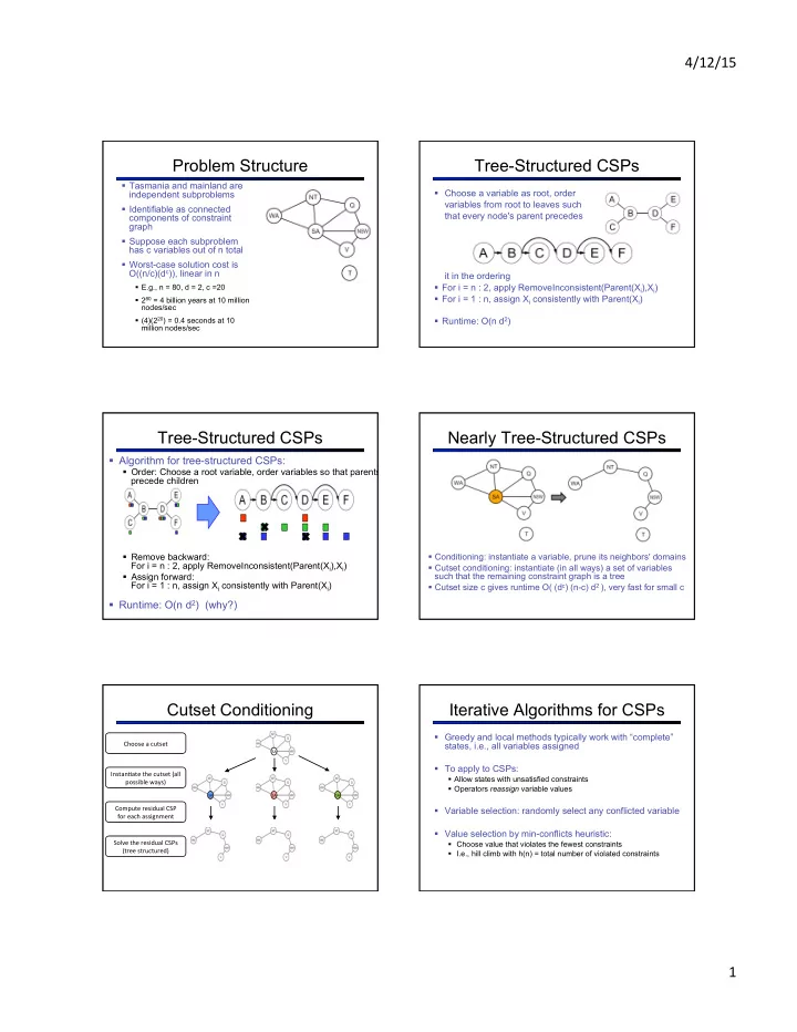
4/12/15 ¡ Problem Structure Tree-Structured CSPs § Tasmania and mainland are independent subproblems § Choose a variable as root, order variables from root to leaves such § Identifiable as connected that every node's parent precedes components of constraint graph § Suppose each subproblem has c variables out of n total § Worst-case solution cost is O((n/c)(d c )), linear in n it in the ordering § For i = n : 2, apply RemoveInconsistent(Parent(X i ),X i ) § E.g., n = 80, d = 2, c =20 § For i = 1 : n, assign X i consistently with Parent(X i ) § 2 80 = 4 billion years at 10 million nodes/sec § (4)(2 20 ) = 0.4 seconds at 10 § Runtime: O(n d 2 ) million nodes/sec Tree-Structured CSPs Nearly Tree-Structured CSPs § Algorithm for tree-structured CSPs: § Order: Choose a root variable, order variables so that parents precede children § Conditioning: instantiate a variable, prune its neighbors' domains § Remove backward: For i = n : 2, apply RemoveInconsistent(Parent(X i ),X i ) § Cutset conditioning: instantiate (in all ways) a set of variables such that the remaining constraint graph is a tree § Assign forward: For i = 1 : n, assign X i consistently with Parent(X i ) § Cutset size c gives runtime O( (d c ) (n-c) d 2 ), very fast for small c § Runtime: O(n d 2 ) (why?) Cutset Conditioning Iterative Algorithms for CSPs § Greedy and local methods typically work with “complete” Choose ¡a ¡cutset ¡ states, i.e., all variables assigned SA ¡ § To apply to CSPs: Instan.ate ¡the ¡cutset ¡(all ¡ § Allow states with unsatisfied constraints possible ¡ways) ¡ § Operators reassign variable values SA ¡ SA ¡ SA ¡ Compute ¡residual ¡CSP ¡ § Variable selection: randomly select any conflicted variable for ¡each ¡assignment ¡ § Value selection by min-conflicts heuristic: Solve ¡the ¡residual ¡CSPs ¡ § Choose value that violates the fewest constraints (tree ¡structured) ¡ § I.e., hill climb with h(n) = total number of violated constraints 1 ¡

4/12/15 ¡ Example: 4-Queens Performance of Min-Conflicts § Given random initial state, can solve n-queens in almost constant time for arbitrary n with high probability (e.g., n = 10,000,000) § The same appears to be true for any randomly-generated CSP except in a narrow range of the ratio § States: 4 queens in 4 columns (4 4 = 256 states) § Operators: move queen in column § Goal test: no attacks § Evaluation: h(n) = number of attacks Summary Local Search § CSPs are a special kind of search problem: States defined by values of a fixed set of variables § § Goal test defined by constraints on variable values § Backtracking = depth-first search with one legal variable assigned per node § Variable ordering and value selection heuristics help significantly § Forward checking prevents assignments that guarantee later failure § Constraint propagation (e.g., arc consistency) does additional work to constrain values and detect inconsistencies § The constraint graph representation allows analysis of problem structure § Tree-structured CSPs can be solved in linear time § Iterative min-conflicts is usually effective in practice Local Search Hill Climbing § Simple, general idea: § Tree search keeps unexplored alternatives on the fringe § Start wherever (ensures completeness) § Repeat: move to the best neighboring state § Local search: improve a single option until you can’t make § If no neighbors better than current, quit it better (no fringe!) § What’s bad about this approach? § New successor function: local changes § Complete? § Optimal? § What’s good about it? § Generally much faster and more memory efficient (but incomplete and suboptimal) 2 ¡

4/12/15 ¡ Hill Climbing Diagram Hill Climbing Star.ng ¡from ¡X, ¡where ¡do ¡you ¡end ¡up ¡? ¡ ¡ ¡ Star.ng ¡from ¡Y, ¡where ¡do ¡you ¡end ¡up ¡? ¡ ¡ Star.ng ¡from ¡Z, ¡where ¡do ¡you ¡end ¡up ¡? ¡ Simulated Annealing Simulated Annealing § Theoretical guarantee: § Idea: Escape local maxima by allowing downhill moves § Stationary distribution: § But make them rarer as time goes on § If T decreased slowly enough, will converge to optimal state! § Is this an interesting guarantee? § Sounds like magic, but reality is reality: § The more downhill steps you need to escape a local optimum, the less likely you are to ever make them all in a row § People think hard about ridge operators which let you jump around the space in better ways 55 Genetic Algorithms Example: N-Queens § Why does crossover make sense here? § When wouldn’t it make sense? § Genetic algorithms use a natural selection metaphor § Keep best N hypotheses at each step (selection) based on a fitness function § What would mutation be? § Also have pairwise crossover operators, with optional mutation to give variety § What would a good fitness function be? § Possibly the most misunderstood, misapplied (and even maligned) technique around 3 ¡

4/12/15 ¡ GA’s for Locomotion Hod Lipson’s Creative Machines Lab @ Cornell 4 ¡