Probability Recap MDM4U: Mathematics of Data Management Determine - - PDF document

SLIDE 1

p r o b a b i l i t y d i s t r i b u t i o n s

MDM4U: Mathematics of Data Management

Accounting For All Probabilities

Probability Distributions

• J. Garvin

Slide 1/16

p r o b a b i l i t y d i s t r i b u t i o n s

Probability Recap

Determine the probability of rolling each possible sum using two six-sided dice. P(2) = 1

36, P(3) = 2 36 = 1 18, P(4) = 3 36 = 1 12,

P(5) = 4

36 = 1 9,

P(6) = 5

36, P(7) = 6 36 = 1 6, P(8) = 5 36, P(9) = 4 36 = 1 9,

P(10) = 3

36 = 1 12, P(11) = 2 36 = 1 18, P(12) = 1 36

• J. Garvin — Accounting For All Probabilities

Slide 2/16

p r o b a b i l i t y d i s t r i b u t i o n s

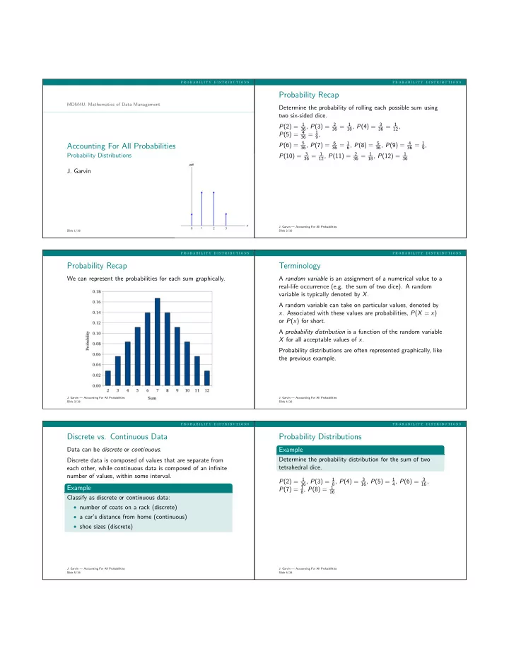
Probability Recap

We can represent the probabilities for each sum graphically.

• J. Garvin — Accounting For All Probabilities

Slide 3/16

p r o b a b i l i t y d i s t r i b u t i o n s

Terminology

A random variable is an assignment of a numerical value to a real-life occurrence (e.g. the sum of two dice). A random variable is typically denoted by X. A random variable can take on particular values, denoted by

• x. Associated with these values are probabilities, P(X = x)
• r P(x) for short.

A probability distribution is a function of the random variable X for all acceptable values of x. Probability distributions are often represented graphically, like the previous example.

• J. Garvin — Accounting For All Probabilities

Slide 4/16

p r o b a b i l i t y d i s t r i b u t i o n s

Discrete vs. Continuous Data

Data can be discrete or continuous. Discrete data is composed of values that are separate from each other, while continuous data is composed of an infinite number of values, within some interval.

Example

Classify as discrete or continuous data:

• number of coats on a rack (discrete)
• a car’s distance from home (continuous)
• shoe sizes (discrete)
• J. Garvin — Accounting For All Probabilities

Slide 5/16

p r o b a b i l i t y d i s t r i b u t i o n s

Probability Distributions

Example

Determine the probability distribution for the sum of two tetrahedral dice. P(2) = 1

16, P(3) = 1 8, P(4) = 3 16, P(5) = 1 4, P(6) = 3 16,

P(7) = 1

8, P(8) = 1 16

• J. Garvin — Accounting For All Probabilities

Slide 6/16

SLIDE 2

p r o b a b i l i t y d i s t r i b u t i o n s

Probability Distributions

• J. Garvin — Accounting For All Probabilities

Slide 7/16

p r o b a b i l i t y d i s t r i b u t i o n s

Uniform Probability Distribution

Some probability distributions are uniform, in that all probabilities are equally likely. For example, consider the probability distribution for the roll

• f a six-sided die.
• J. Garvin — Accounting For All Probabilities

Slide 8/16

p r o b a b i l i t y d i s t r i b u t i o n s

Uniform Probability Distribution

• J. Garvin — Accounting For All Probabilities

Slide 9/16

p r o b a b i l i t y d i s t r i b u t i o n s

Uniform Probability Distribution

Probability in a Uniform Probability Distribution

For a uniform probability distribution, p(x), with n possible

• utcomes, the probability of each outcome is P(x) = 1

n. This should be intuitive. Imagine a spinner divided into n equally-sized sectors. Each outcome is equally likely, and a player has a 1 in n chance of landing in any given sector.

• J. Garvin — Accounting For All Probabilities

Slide 10/16

p r o b a b i l i t y d i s t r i b u t i o n s

Expected Value

In many cases, we are interested in knowing what value we can expect as an outcome. The expected value, denoted E(X), is the predicted average

• f all possible outcomes in an experiment.

Expected Value for a Discrete Probability Distribution

E(X) = x1P(x1) + x2P(x2) + . . . + xnP(xn)

• r using sigma notation. . .

E(X) =

n

• i=1

xiP(xi)

• J. Garvin — Accounting For All Probabilities

Slide 11/16

p r o b a b i l i t y d i s t r i b u t i o n s

Expected Value

Example

What is the expected sum when two dice are rolled? Solution: Create a table of values, to calculate the expected value for each roll. Roll Prob. xP(x) 2

1 36 2 36

3

2 36 6 36

4

3 36 12 36

5

4 36 20 36

6

5 36 30 36

7

6 36 42 36

Roll Prob. xP(x) 8

5 36 40 36

9

4 36 36 36

10

3 36 30 36

11

2 36 22 36

12

1 36 12 36

So the expected valus is E(X) =

n

• i=1

xiP(xi) = 7.

• J. Garvin — Accounting For All Probabilities

Slide 12/16

SLIDE 3

p r o b a b i l i t y d i s t r i b u t i o n s

Fairness

A fair game must not be biased toward a particular player. If the expected value of a game is negative, it may represent a loss for a player, while a positive expected value may represent a win. The expected value of a fair game is zero.

• J. Garvin — Accounting For All Probabilities

Slide 13/16

p r o b a b i l i t y d i s t r i b u t i o n s

Fairness

Example

Three coins are tossed. If an even number of heads is tossed, the player wins $5. If an odd number of heads is tossed, the player loses $3. Is the game fair? Create a table of values, to calculate the expected value for each sequence of tosses. Heads Outcomes Probability Payout xP(x) TTT

1 8

5

5 8

1 HTT, THT, TTH

3 8

• 3

− 9

8

2 HHT, HTH, THH

3 8

5

15 8

3 HHH

1 8

• 3

− 3

8

So E(X) =

n

• i=0

xiP(xi) = 1.

• J. Garvin — Accounting For All Probabilities

Slide 14/16

p r o b a b i l i t y d i s t r i b u t i o n s

Fairness

On average, a player can expect to win $1 each round. The game is not fair, but biased toward the player. To visualize, imagine a game where four rounds are played. Since it is equally likely to get an even number of heads as it is an odd number, both results should occur roughly half the time each. So for a four round game, a player would be expected to win $5 twice, and lose $3 twice, for a net gain of $4. This is equivalent to $1 per round.

• J. Garvin — Accounting For All Probabilities

Slide 15/16

p r o b a b i l i t y d i s t r i b u t i o n s

Questions?

• J. Garvin — Accounting For All Probabilities

Slide 16/16