Probability and Statistics for Computer Science Its straigh+orward - - PowerPoint PPT Presentation

ì

Probability and Statistics for Computer Science

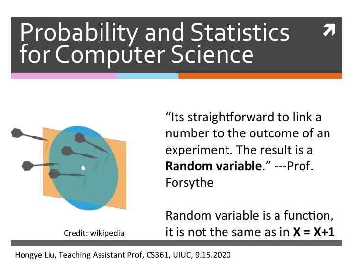
“Its straigh+orward to link a number to the outcome of an

• experiment. The result is a

Random variable.” ---Prof. Forsythe Random variable is a funcCon, it is not the same as in X = X+1

Hongye Liu, Teaching Assistant Prof, CS361, UIUC, 9.15.2020 Credit: wikipedia

Last time

Which is larger?

Random numbers

✺ Amount of money on a bet ✺ Age at reCrement of a populaCon ✺ Rate of vehicles passing by the toll ✺ Body temperature of a puppy in its pet clinic ✺ Level of the intensity of pain in a toothache

Random variable as vectors

• A. McDonald et al. NeuroImage doi: 10.1016/

j.neuroimage.2016.10.048

Brain imaging

• f Human

emoCons A) Moral conflict B) MulC-task C) Rest

Content

✺ Random Variable

Random variables

Random variables

✺ The values of a random variable can

be either discrete, con5nuous or mixed.

Discrete Random variables

✺ The range of a discrete random

variable is a countable set of real numbers.

Random Variable Example

✺ Number of pairs in a hand of 5 cards

✺ Let a single outcome be the hand of 5 cards ✺ Each outcome maps to values in the set of

numbers {0, 1, 2}

Random Variable Example

✺ Number of pairs in a hand of 6 cards ✺ Let a single outcome be the hand

• f 6 cards

✺ What is the range of values of this

random variable?

Q: Random Variable

✺ If we roll a 3-sided fair die, and define

random variable U, such that

• A. {-1, 0, 1}
• B. {0, 1}

Three important facts of Random variables

✺ Random variables have

probability func5ons

✺ Random variables can be

condi5oned on events or other random variables

✺ Random variables have averages

Random variables have probability functions

✺ Let X be a random variable ✺ The set of outcomes

is an event with probability X is the random variable is any unique instance that X takes on

Probability Distribution

✺ is called the probability

distribuCon for all possible x

✺ is also denoted as or ✺ for all values that X can

take, and is 0 everywhere else

✺ The sum of the probability

distribuCon is 1

P(X = x) P(x) P(X = x)

p(x)

P(X = x) ≥ 0

• x

P(x) = 1

Examples of Probability Distributions

Cumulative distribution

✺ is called the cumulaCve

distribuCon funcCon of X

✺ is also denoted as ✺ is a non-decreasing

funcCon of x

P(X ≤ x)

f(x)

P(X ≤ x) P(X ≤ x)

Probability distribution and cumulative distribution

✺ Give the random variable X,

X

1 1/2

X(ω) =

• 1
• utcome of ω is head
• utcome of ω is tail

p(x)

X

1 1/2 1

f(x)

P(X = x) P(X ≤ x)

Functions of random variables

• Q. Are these random variables the same?

Function of random variables: die example

2 3 4 2 3 4 1 1

Roll 4-sided fair die twice. Define these random variables: X, the values of 1st roll Y, the values of 2nd roll Sum S = X + Y Difference D= X - Y

X Y

Size of Sample Space = ?

Random variable: die example

2 3 4 2 3 4 1 1

Roll 4-sided fair die twice.

X Y

Size of Sample Space = 16

x

P(X = 1) P(Y ≤ 2) P(S = 7) P(D ≤ −1)

Random variable: die example

2 3 4 2 3 4 1 1

Roll 4-sided fair die twice.

X Y

Size of Sample Space = 16

x

P(X = 1) P(Y ≤ 2) P(S = 7) P(D ≤ −1)

1 4

1 2

Random variable: die example

2 3 4 2 3 4 1 1

X Y

P(S = 7) P(D ≤ −1)

2 3 4 2 3 4 1 1

X Y S = X + Y D = X-Y

2 3 4 5 3 4 5 6 4 5 6 5 6 7 8

• 3 -2
• 1 0
• 2 -1

1

• 1 0

1 2 1 2 3 7

Probability distribution of the sum

• f two random variables

✺ Give the random variable S in the 4-

sided die, whose range is {2,3,4,5,6,7,8}, probability distribuCon of S.

S

2 3 4 5 6 7 8

p(s)

1/16

Probability distribution of the difference of two random variables

✺ Give the random variable D = X-Y,

what is the probability distribu<on of D?

1/16

Conditional Probability

✺ The probability of A given B

Credit: Prof. Jeremy Orloff & Jonathan Bloom

P(A|B) = P(A ∩ B) P(B)

P(B) ̸= 0

The “Size” analogy

• x

P(x|y) = 1

Conditional probability distribution

• f random variables

✺ The condiConal probability distribuCon

• f X given Y is

P(x|y) = P(x, y) P(y) P(y) ̸= 0

Conditional probability distribution

• f random variables

✺ The condiConal probability distribuCon

• f X given Y is

✺ The joint probability distribuCon of two

random variables X and Y is

P(x|y) = P(x, y) P(y) P(y) ̸= 0

P({X = x} ∩ {Y = y})

• x

P(x|y) = 1

Get the marginal from joint distri.

✺ We can recover the individual

probability distribuCons from the joint probability distribuCon

P(x) =

• y

P(x, y)

P(y) =

• x

P(x, y)

Joint probabilities sum to 1

✺ The sum of the joint probability

distribuCon

• y
• x

P(x, y) = 1

Joint Probability Example

✺ Tossing a coin twice, we define

random variable X and Y for each toss.

X(ω) =

• 1
• utcome of ω is head
• utcome of ω is tail

Y (ω) =

• 1
• utcome of ω is head
• utcome of ω is tail

Joint probability distribution example

1

X Y

P(x, y)

P(x)

P(y)

1

Joint Probability Example

Now we define Sum S = X + Y, Difference D = X – Y. S takes on values {0,1,2} and D takes on values {-1, 0, 1}

X(ω) =

• 1
• utcome of ω is head
• utcome of ω is tail

Y (ω) =

• 1
• utcome of ω is head
• utcome of ω is tail

Joint Probability Example

X =1 X =0 Y =1 Y =0 Y =1 Y =0

S D

2 1 1 1

• 1

P(s, d) 1st toss 2nd toss Suppose coin is fair, and the tosses are independent

Joint probability distribution example

1 2 1

• 1

D S P(s, d)

P(s)

P(d)

Independence of random variables

✺ Random variable X and Y are

independent if

✺ In the previous coin toss example ✺ Are X and Y independent? ✺ Are S and D independent?

P(x, y) = P(x)P(y) for all x and y

Joint probability distribution example

1

X Y

P(x, y)

P(x)

P(y)

1

1 4 1 4 1 4 1 4 1 2 1 2 1 2 1 2

Joint probability distribution example

1 2 1

• 1

D S

1 4 1 4 1 4 1 4 1 4 1 4

1 2

P(s, d)

P(s)

P(d)

1 4 1 4

1 2

Conditional probability distribution example

1 2 1

• 1

D S

P(s|d) = P(s, d) P(d)

1 2 1 2

1 1

Bayes rule for random variable

✺ Bayes rule for events generalizes to

random variables

P(A|B) = P(B|A)P(A) P(B)

P(x|y) = P(y|x)P(x) P(y)

= P(y|x)P(x)

• x P(y|x)P(x)

Total Probability

Conditional probability distribution example

1 2 1

• 1

D S

P(s|d) = P(s, d) P(d)

1 2 1 2

1 1

P(D = −1|S = 1) = P(S = 1|D = −1)P(D = −1) P(S = 1)

1 × 1

4 1 2

=

Assignments

✺ Chapter 4 of the textbook ✺ Next Cme: More random variable,

ExpectaCons, Variance

Additional References

✺ Charles M. Grinstead and J. Laurie Snell

"IntroducCon to Probability”

✺ Morris H. Degroot and Mark J. Schervish

"Probability and StaCsCcs”

See you next time

See You!