Probability and Statistics for Computer Science The - - PowerPoint PPT Presentation

ì ¡

Probability ¡and ¡Statistics ¡ for ¡Computer ¡Science ¡ ¡

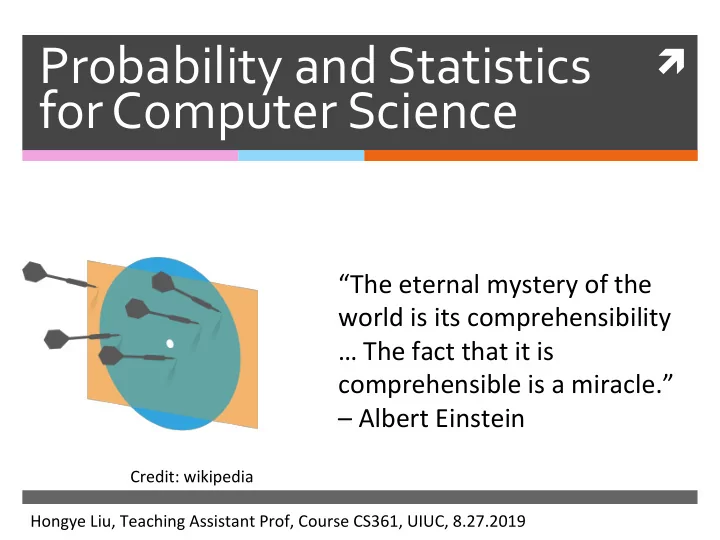
“The ¡eternal ¡mystery ¡of ¡the ¡ world ¡is ¡its ¡comprehensibility … The ¡fact ¡that ¡it ¡is ¡ comprehensible ¡is ¡a ¡miracle.” ¡ – ¡Albert ¡Einstein ¡

Hongye ¡Liu, ¡Teaching ¡Assistant ¡Prof, ¡Course ¡CS361, ¡UIUC, ¡8.27.2019 ¡ Credit: ¡wikipedia ¡

Contents ¡

✺ Course ¡materials ¡and ¡course ¡staff ¡ ✺ Overview ¡of ¡CS361 ¡ ✺ Lecture ¡1 ¡-­‑ ¡Data ¡VisualizaXon ¡& ¡

Summary ¡(I) ¡ ¡

Course ¡materials ¡and ¡course ¡staff ¡

✺ Website ¡& ¡Survey ¡ ✺ Meet ¡our ¡TAs ¡and ¡GA ¡

¡Anay, ¡Andrew, ¡Ehsan, ¡Umar ¡ ¡& ¡Emma! ¡ ¡

✺ Cell ¡phone, ¡laptop ¡policy ¡

¡ ¡

Course ¡materials ¡and ¡course ¡staff ¡

✺ Website ¡& ¡Survey ¡

h`ps://courses.engr.illinois.edu/cs361/ fa2019/ ¡ ¡ ¡ ¡ ¡(more ¡to ¡be ¡updated ¡such ¡as ¡office ¡hours) ¡ ¡Test ¡iClicker ¡… ¡

Course ¡materials ¡and ¡course ¡staff ¡

✺ Have ¡you ¡done ¡the ¡survey ¡on ¡the ¡course ¡

website? ¡ ¡A. ¡Yes. ¡ ¡ ¡ ¡B. ¡No. ¡

Cell ¡phone ¡& ¡laptop ¡policy ¡in ¡lecture ¡

✺ Cell ¡phone ¡is ¡expected ¡to ¡be ¡silenced ¡and ¡

put ¡away ¡unless ¡permi`ed ¡by ¡the ¡ instructor ¡

✺ Laptop ¡is ¡allowed ¡to ¡be ¡used, ¡but ¡laptop ¡

users ¡are ¡suggested ¡to ¡sit ¡relaXvely ¡toward ¡ the ¡back ¡so ¡that ¡non-­‑users ¡won’t ¡get ¡

• disturbed. ¡Its ¡usage ¡should ¡be ¡course ¡

lecture ¡related ¡such ¡as ¡taking ¡notes, ¡etc. ¡ ¡

Meet ¡Our ¡Staff ¡

Instructor: ¡Hongye ¡Liu ¡ Teaching ¡Assistants: ¡Anay ¡Pa`anaik, ¡ ¡ ¡ ¡ ¡ ¡ ¡ ¡ ¡Andrew ¡Yoo, ¡ ¡ ¡ ¡ ¡ ¡ ¡ ¡ ¡Ehsan ¡Saleh, ¡ ¡ ¡ ¡ ¡ ¡ ¡ ¡Umar ¡Farooq ¡ ¡ Graduate ¡Assistant: ¡ ¡Emma ¡Marie ¡Taylor ¡ We ¡will ¡have ¡course ¡grading ¡assistants ¡

• later. ¡ ¡ ¡

Overview ¡of ¡CS361 ¡

✺ Probability ¡and ¡StaXsXcs ¡in ¡acXon ¡ ✺ What ¡does ¡this ¡course ¡teach? ¡

¡Textbook: ¡Forsyth, ¡D. ¡A. ¡"Probability ¡and ¡Sta@s@cs ¡for ¡Computer ¡ ¡Science," ¡Springer ¡(2018) ¡

✺ Why ¡are ¡there ¡4 ¡secXons? ¡How ¡are ¡

they ¡related? ¡

✺ Learning ¡Programming ¡R ¡

This ¡field ¡really ¡started ¡with ¡gaming ¡

✺ We ¡are ¡familiar ¡with ¡flipping ¡a ¡

coin ¡or ¡throwing ¡a ¡dice, ¡the ¡ result ¡is ¡uncertain! ¡

Head ¡ ¡ Or ¡Tail? ¡ Which ¡side ¡ ¡is ¡front? ¡

Life ¡is ¡uncertain ¡so ¡aim ¡for ¡long-­‑ term ¡average ¡

✺ We ¡repeat ¡a ¡lot ¡of ¡experiments ¡

and ¡see ¡if ¡there ¡is ¡regularity ¡

Head ¡ ¡ Or ¡Tail? ¡ Which ¡side ¡ ¡is ¡front? ¡

Throwing ¡a ¡lot ¡of ¡“coins” ¡for ¡many ¡ times ¡in ¡one ¡touch ¡

✺ Galton ¡board, ¡the ¡Bead ¡Machine ¡

¡h`ps://www.youtube.com/watch? v=Kq7e6cj2nDw ¡ ¡ ¡

Probability ¡and ¡Statistics ¡ Experiment ¡in ¡action ¡

✺ Try ¡the ¡bead ¡machine ¡4 ¡Xmes, ¡the ¡

first ¡two ¡runs ¡with ¡the ¡base ¡on ¡the ¡ table, ¡the ¡next ¡2 ¡runs ¡however ¡you ¡ like ¡as ¡long ¡as ¡you ¡don’t ¡break ¡it. ¡

✺ I ¡will ¡ask ¡you ¡some ¡simple ¡quesXons ¡

later ¡on. ¡ ¡

Simulation ¡of ¡random ¡draw ¡of ¡a ¡ picture ¡on ¡computer ¡

✺ It’s ¡the ¡same ¡as ¡ ¡

throwing ¡a ¡4-­‑sided ¡die. ¡ ¡

Assign ¡logos ¡ ¡

Group1 ¡ Group3 ¡ Group2 ¡ Group4 ¡

Break ¡

What ¡does ¡this ¡course ¡teach? ¡

✺ Describing ¡Datasets ¡

¡Summary ¡& ¡visualizaXon ¡

✺ Probability ¡ ¡ ✺ Inference ¡– ¡StaXsXcal ¡Inference ¡ ✺ Tools ¡– ¡Machine ¡Learning ¡tools ¡

Describing ¡datasets ¡(Summary ¡& ¡ visualization ¡) ¡

¡Descrip(ve ¡& ¡Graphical ¡ ¡

SummarizaXon ¡of ¡4 ¡locaXons’ ¡annual ¡mean ¡ ¡ temperature ¡by ¡month ¡

Probability ¡ ¡

✺ Mathema@cal ¡

Romeo ¡and ¡Juliet ¡have ¡a ¡date ¡ Each ¡arrives ¡with ¡a ¡delay ¡btw ¡0 ¡and ¡1 ¡

• hour. ¡The ¡first ¡to ¡arrive ¡leaves ¡arer ¡1/4 ¡
• hour. ¡All ¡pairs ¡of ¡delays ¡are ¡equally ¡likely. ¡

What's ¡the ¡probability ¡that ¡they ¡will ¡ meet? ¡ ¡

Inference ¡

✺ Analy@cal ¡

Treatment ¡1 ¡ Treatment ¡2 ¡ ¡ ¡ ¡ ¡ ¡ ¡ ¡ ¡ ¡ ¡ ¡ ¡ ¡ ¡ ¡ ¡ ¡ ¡ ¡ ¡ ¡ ¡

How ¡different ¡ ¡ are ¡they? ¡

J ¡Fromonot ¡et ¡al ¡ JACC ¡2016 ¡

Tools ¡(Machine ¡learning) ¡

✺ Algorithmical ¡

High-­‑dimensional ¡or ¡ ¡ complex ¡shaped ¡ data ¡sets ¡need ¡tools! ¡ ¡ Humans ¡are ¡limited ¡in ¡ 2-­‑3D. ¡ Machine ¡learning ¡is ¡ ¡ Highly ¡desired! ¡ Oren ¡depends ¡on ¡ ¡

• StaXsXcs. ¡

Cancer ¡Cell ¡Division ¡Clusters ¡

Different ¡human ¡cells ¡

Why ¡these ¡4 ¡sections? ¡

✺ Summary ¡& ¡visualizaXon ¡

Graphical ¡

✺ Probability ¡ ¡

Mathema@cal ¡

✺ Inference ¡– ¡StaXsXcal ¡Inference ¡

Analy@cal ¡

✺ Tools ¡– ¡Machine ¡Learning ¡tools ¡

Algorithmical ¡

Why ¡these ¡4 ¡sections? ¡

✺ The ¡common ¡thread ¡is ¡Data. ¡ ¡ ✺ We ¡are ¡doing ¡computer ¡science ¡and ¡so ¡

are ¡like ¡ these ¡ yellow ¡ ¡ fish ¡

¡ StaXsXcs ¡ MathemaXcs ¡ ¡ Data ¡Science ¡+ ¡

• Comp. ¡Science ¡

Why ¡these ¡4 ¡sections? ¡

✺ Real ¡world ¡data ¡is ¡oren ¡high ¡

dimensional ¡and ¡complex ¡

✺ These ¡4 ¡parts ¡of ¡knowledge ¡or ¡

techniques ¡are ¡inseparably/

• rganically ¡connected ¡in ¡many ¡real ¡

world ¡applicaXons. ¡

Learning ¡Programming ¡R ¡

✺ Language ¡of ¡the ¡staXsXcians ¡ ✺ Best-­‑in-­‑class ¡visualizaXon ¡tools ¡ ✺ Countless ¡expert ¡packages ¡

including ¡machine ¡learning ¡

✺ Open-­‑source, ¡free ¡

Which ¡are ¡the ¡success ¡ingredients? ¡

• A. Try ¡your ¡best ¡to ¡be ¡engaged, ¡learn ¡from ¡

the ¡course ¡and ¡from ¡each ¡other, ¡ ¡

• B. AcXve ¡in ¡class ¡parXcipaXon ¡
• C. Do ¡as ¡much ¡pracXce ¡as ¡possible, ¡not ¡just ¡

the ¡homework. ¡

• D. Read ¡the ¡textbook ¡
• E. All ¡the ¡above ¡
• F. Why ¡does ¡i-­‑clicker ¡have ¡only ¡5 ¡choices? ¡

Which ¡are ¡the ¡success ¡ingredients? ¡

• A. Try ¡your ¡best ¡to ¡be ¡engaged, ¡learn ¡from ¡

the ¡course ¡and ¡from ¡each ¡other, ¡ ¡

• B. AcXve ¡in ¡class ¡parXcipaXon ¡
• C. Do ¡as ¡much ¡pracXce ¡as ¡possible, ¡not ¡just ¡

the ¡homework. ¡

• D. Read ¡the ¡textbook ¡
• E. All ¡the ¡above ¡
• F. Why ¡does ¡i-­‑clicker ¡have ¡only ¡5 ¡choices? ¡

Break ¡

Lecture ¡I: ¡Data ¡Visualization ¡ &Summary ¡

✺ Datasets ¡{x} ¡– ¡a ¡set ¡of ¡N ¡items ¡xi, ¡

i=1…N, ¡each ¡of ¡which ¡is ¡a ¡tuple ¡ ¡

Each ¡row ¡ ¡is ¡a ¡tuple ¡ ¡ Proteins ¡ Cells ¡

Lecture ¡I: ¡Data ¡Visualization ¡ &Summary ¡

✺ ConvenXon: ¡columns ¡are ¡the ¡features; ¡the ¡

number ¡of ¡features ¡is ¡dimension. ¡

Each ¡row ¡ ¡is ¡a ¡tuple ¡with ¡dimension ¡=5 ¡ ¡ Proteins ¡ Cells ¡

Data ¡types ¡

✺ Categorical ¡ ✺ Ordinal ¡ ✺ ConXnuous ¡

Data ¡types ¡

✺ Categorical ¡

Smoker ¡or ¡non-­‑Smoker, ¡Female ¡or ¡Male ¡etc. ¡ ¡ ¡ ¡

✺ Ordinal ¡

Not ¡saXsfied, ¡saXsfied, ¡very ¡saXsfied ¡

✺ ConXnuous ¡(any ¡real ¡number ¡within ¡a ¡range) ¡

Temperature ¡

Simple ¡Visualization ¡of ¡Data ¡ ¡

¡

✺ General ¡principles ¡ ✺ Bar ¡chart ¡ ✺ Histogram ¡ ✺ CondiXonal ¡histogram ¡

Simple ¡Visualization ¡of ¡Data ¡ ¡

✺ Tables ¡

¡In ¡R, ¡there ¡is ¡table ¡format ¡and ¡there ¡ is ¡data.frame ¡which ¡is ¡a ¡very ¡versaXle ¡ table ¡for ¡storing ¡all ¡kinds ¡of ¡data ¡type. ¡

Simple ¡Visualization ¡of ¡Data ¡ ¡

¡

✺ General ¡principles ¡

¡Must ¡not ¡mislead ¡or ¡distort; ¡ ¡AestheXcally ¡pleasing; ¡ ¡Clear, ¡A`racXve, ¡Convincing; ¡ ¡Show ¡message/significance. ¡

Simple ¡Visualization ¡of ¡Data ¡ ¡

✺ Bar ¡chart ¡

¡ ¡

A ¡set ¡of ¡bars ¡that ¡ are ¡organized ¡ ¡ by ¡categorical ¡

• r ¡ordinal ¡feature ¡

Data: ¡“mtcars” ¡in ¡R ¡

An ¡example ¡of ¡good, ¡ugly, ¡bad, ¡wrong ¡

• C. ¡Wilke ¡“Fundamentals ¡of ¡Data ¡VisualizaXon” ¡
• Dr. ¡Wilke ¡

illustrated ¡the ¡ difference ¡ between ¡good, ¡ ugly, ¡bad ¡and ¡ wrong ¡ visualiza(on ¡

Q: ¡Is ¡this ¡a ¡good ¡bar ¡chart? ¡

• A. Yes ¡ ¡ ¡ ¡
• B. ¡ ¡No ¡

How ¡about ¡using ¡a ¡color ¡scale ¡

Simple ¡Visualization ¡of ¡Data ¡ ¡

✺ Histogram ¡

A ¡set ¡of ¡bars ¡that ¡ are ¡organized ¡ ¡ by ¡bins ¡that ¡ contains ¡ numerical ¡data ¡ (discrete ¡or ¡ con?nuous) ¡

Data: ¡“iris” ¡in ¡R ¡

Simple ¡Visualization ¡of ¡Data ¡ ¡

✺ CondiXonal ¡ ¡

histogram ¡

Histogram ¡ generated ¡by ¡ subsets ¡of ¡the ¡ data ¡

Data: ¡“iris” ¡in ¡R ¡

Smoothed ¡Histogram ¡in ¡R ¡

✺ Averaged ¡ ¡ ¡

Shired ¡Histogram ¡ in ¡R ¡using ¡ash1(). ¡ ¡

Summarizing ¡1D ¡continuous ¡data ¡

✺ LocaXon ¡Parameters ¡

✺ Mean ¡ ¡ ✺ Median ¡ ✺ Mode ¡

✺ Scale ¡parameters ¡

✺ Standard ¡deviaXon ¡and ¡variance ¡ ✺ InterquarXle ¡range ¡

Summarizing ¡1D ¡continuous ¡data ¡ ¡

✺ Mean ¡

¡ ¡ ¡ mean(xi) = 1 N

N

• i=1

xi

It’s ¡the ¡centroid ¡of ¡the ¡data ¡geometrically, ¡ by ¡idenXfying ¡the ¡data ¡set ¡at ¡that ¡point, ¡you ¡find ¡ ¡ the ¡center ¡of ¡balance. ¡

Properties ¡of ¡the ¡mean ¡

✺ Scaling ¡data ¡scales ¡the ¡mean ¡ ✺ TranslaXng ¡the ¡data ¡translates ¡the ¡mean ¡

¡ ¡ ¡

mean({k · xi}) = k · mean({xi})

mean({xi + c}) = mean({xi}) + c

Less ¡obvious ¡properties ¡of ¡the ¡mean ¡

✺ The ¡signed ¡distances ¡from ¡the ¡mean ¡ ¡

¡sum ¡to ¡0 ¡

✺ The ¡mean ¡minimizes ¡the ¡sum ¡of ¡the ¡

squared ¡distance ¡from ¡the ¡mean ¡ ¡ ¡ ¡

N

• i=1

(xi − mean({xi})) = 0

argmin

µ N

• i=1

(xi − µ)2 = mean({xi})

Qs: ¡

¡

✺ What ¡is ¡the ¡answer ¡for ¡

¡mean(mean({xi})) ¡? ¡ ¡ ¡

¡

¡ ¡

✺ Recall ¡in ¡which ¡applicaXon ¡did ¡we ¡

compare ¡the ¡means ¡of ¡experiments? ¡

• A. ¡mean({xi}) ¡ ¡ ¡ ¡B. ¡unsure ¡ ¡ ¡C. ¡0 ¡

Standard ¡Deviation ¡

¡

✺ The ¡standard ¡deviaXon ¡

std({xi}) =

• 1

N

N

• i=1

(xi − mean({xi}))2

std({xi}) =

• mean({xi − mean({xi}))2})

Properties ¡of ¡the ¡standard ¡deviation ¡

✺ Scaling ¡data ¡scales ¡the ¡standard ¡deviaXon ¡ ✺ TranslaXng ¡the ¡data ¡does ¡NOT ¡change ¡the ¡

standard ¡deviaXon ¡ ¡ ¡ ¡ std({k · xi}) = |k| · std({xi})

std({xi + c}) = std({xi})

Standard ¡deviation: ¡Chebyshev’s ¡ inequality ¡

✺ At ¡most ¡ ¡ ¡ ¡ ¡ ¡items ¡are ¡k ¡standard ¡

deviaXons ¡(σ) ¡away ¡from ¡the ¡mean ¡

✺ Rough ¡jusXficaXon: ¡Assume ¡mean ¡=0 ¡

N k2

0 ¡

N − N K2

0.5N K2 0.5N K2

−kσ

kσ

std =

• 1

N [(N − N k )02 + N k2(kσ)2] = σ

Reading ¡for ¡this ¡week ¡

✺ We ¡will ¡post ¡notes ¡and ¡codes ¡arer ¡each ¡

lecture ¡

✺ Chapter ¡1 ¡of ¡the ¡text ¡book ¡

Textbook: ¡Forsyth, ¡D. ¡A. ¡"Probability ¡and ¡ Sta@s@cs ¡for ¡Computer ¡ ¡Science," ¡Springer ¡ (2018) ¡

Additional ¡References ¡

✺ Peter ¡Dalgaard ¡"Introductory ¡StaXsXcs" ¡

with ¡R ¡

✺ Charles ¡M. ¡Grinstead ¡and ¡J. ¡Laurie ¡Snell ¡

"IntroducXon ¡to ¡Probability” ¡ ¡

✺ Morris ¡H. ¡Degroot ¡and ¡Mark ¡J. ¡Schervish ¡

"Probability ¡and ¡StaXsXcs” ¡

See ¡you ¡next ¡time ¡

See you!