Practical aspects of prediction in Mortality CVD event multistate - - PDF document

Practical aspects of prediction in multistate models

Bendix Carstensen

Steno Diabetes Center, Gentofte, Denmark

& Department of Biostatistics, University of Copenhagen

bxc@steno.dk http://BendixCarstensen.com FRIAS, Freiburg Germany, 21–23 September 2016 http://BendixCarstensen/AdvCoh/Frias-2016

1/ 26

ARTICLE

Years of life gained by multifactorial intervention in patients with type 2 diabetes mellitus and microalbuminuria: 21 years follow-up on the Steno-2 randomised trial

Peter Gæde1,2 & Jens Oellgaard1,2,3 & Bendix Carstensen3 & Peter Rossing3,4,5 & Henrik Lund-Andersen3,5,6 & Hans-Henrik Parving5,7 & Oluf Pedersen8

Received: 7 April 2016 /Accepted: 1 July 2016 # The Author(s) 2016. This article is published with open access at Springerlink.com

Abstract Aims/hypothesis The aim of this work was to study the poten- tial long-term impact of a 7.8 years intensified, multifactorial pharmacological approaches. After 7.8 years the study contin- ued as an observational follow-up with all patients receiving treatment as for the original intensive-therapy group. The pri-

Diabetologia DOI 10.1007/s00125-016-4065-6

2/ 26 DM 1,108.2 80 28 1st CVD 132.3 5 2nd CVD 44.7 5 3+ CVD 24.7 4 D(no CVD) 17 D(1 CVD) 13 D(2 CVD) 5 D(3+ CVD) 3 35 (3.2) 17 (1.5) 17 (12.9) 13 (9.8) 7 (15.7) 5 (11.2) 3 (12.1) DM 1,108.2 80 28 1st CVD 132.3 5 2nd CVD 44.7 5 3+ CVD 24.7 4 D(no CVD) 17 D(1 CVD) 13 D(2 CVD) 5 D(3+ CVD) 3 DM 1,108.2 80 28 1st CVD 132.3 5 2nd CVD 44.7 5 3+ CVD 24.7 4 D(no CVD) 17 D(1 CVD) 13 D(2 CVD) 5 D(3+ CVD) 3 Intensive DM 762.5 80 13 1st CVD 210.3 6 2nd CVD 67.6 2 3+ CVD 67.4 4 D(no CVD) 16 D(1 CVD) 14 D(2 CVD) 11 D(3+ CVD) 14 51 (6.7) 16 (2.1) 31 (14.7) 14 (6.7) 17 (25.2) 11 (16.3) 14 (20.8) DM 762.5 80 13 1st CVD 210.3 6 2nd CVD 67.6 2 3+ CVD 67.4 4 D(no CVD) 16 D(1 CVD) 14 D(2 CVD) 11 D(3+ CVD) 14 DM 762.5 80 13 1st CVD 210.3 6 2nd CVD 67.6 2 3+ CVD 67.4 4 D(no CVD) 16 D(1 CVD) 14 D(2 CVD) 11 D(3+ CVD) 14 Conventional 3/ 26

DM 1,108.2 80 28 1st CVD 132.3 5 2nd CVD 44.7 D(no CVD) 17 D(1 CVD) 13 D(2 CVD) 5 35 (3.2) 17 (1.5) 17 (12.9) 13 (9.8) 5 (11.2) DM 1,108.2 80 28 1st CVD 132.3 5 2nd CVD 44.7 D(no CVD) 17 D(1 CVD) 13 D(2 CVD) 5 DM 1,108.2 80 28 1st CVD 132.3 5 2nd CVD 44.7 D(no CVD) 17 D(1 CVD) 13 D(2 CVD) 5 Intensive DM 762.5 80 13 1st CVD 210.3 6 2nd CVD 67.6 D(no CVD) 16 D(1 CVD) 14 D(2 CVD) 11 51 (6.7) 16 (2.1) 31 (14.7) 14 (6.7) 11 (16.3) DM 762.5 80 13 1st CVD 210.3 6 2nd CVD 67.6 D(no CVD) 16 D(1 CVD) 14 D(2 CVD) 11 DM 762.5 80 13 1st CVD 210.3 6 2nd CVD 67.6 D(no CVD) 16 D(1 CVD) 14 D(2 CVD) 11 Conventional

4/ 26

Hazard ratios

Mortality CVD event HR, Int. vs. Conv. 0.83(0.54; 1.30) 0.55(0.39;0.77) H0: PH btw. CVD groups p=0.438 p=0.261 H0: HR = 1 p=0.425 p=0.001 HR vs. 0 CVD events: 0 (ref.) 1.00 1.00 1 3.08(1.82; 5.19) 2.43(1.67;3.52) 2 4.42(2.36; 8.29) 3.48(2.15;5.64) 3+ 7.76(4.11;14.65)

5/ 26 5 10 15 20 0.0 0.2 0.4 0.6 0.8 1.0 Probability 0.0 0.2 0.4 0.6 0.8 1.0 Intensive 20 15 10 5 Conventional Time since baseline (years) 6/ 26

between groups (HR 0.83 [95% CI 0.54, 1.30], p=0.43). Thus, the reduced mortality was primarily due to reduced risk of CVD. The patients in the intensive group experienced a total of 90 cardiovascular events vs 195 events in the conventional

• group. Nineteen intensive-group patients (24%) vs 34

conventional-group patients (43%) experienced more than

• ne cardiovascular event. No significant between-group dif-

ference in the distribution of specific cardiovascular first- event types was observed (Table 2 and Fig. 4). Microvascular complications Hazard rates of progression rates in microvascular complications compared with baseline status are shown Fig. 3. Sensitivity analyses showed a negli- gible effect of the random dates imputation. Progression of retinopathy was decreased by 33% in the intensive-therapy group (Fig. 5). Blindness in at least one eye was reduced in the intensive-therapy group with an HR of 0.47 (95% CI 0.23, 0.98, p=0.044). Autonomic neuropathy was decreased by 41% in the intensive-therapy group (Fig. 5). We

• bserved no difference between groups in the progression of

peripheral neuropathy (Fig. 5). Progression to diabetic ne- phropathy (macroalbuminuria) was reduced by 48% in the intensive-therapy group (Fig. 5). Ten patients in the conventional-therapy groups vs five patients in the intensive- therapy group progressed to end-stage renal disease (p=0.061). Discussion

a

25 50 75 100 Cumulative mortality (%) 80 78 65 45 34 24 Conventional 80 76 66 58 54 43 Intensive Number at risk 4 8 12 16 20 Years since randomisation

b

25 50 75 100 Death or CVD event (%) 80 61 40 27 18 13 Conventional 80 66 56 49 41 31 Intensive Number at risk 4 8 12 16 20 Years since randomisation

7/ 26

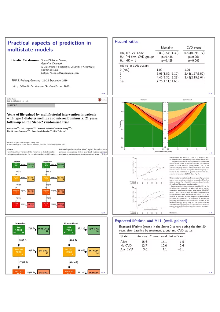
Expected lifetime and YLL (well, gained)

Expected lifetime (years) in the Steno 2 cohort during the first 20 years after baseline by treatment group and CVD status. State Intensive Conventional Int.−Conv. Alive 15.6 14.1 1.5 No CVD 12.7 10.0 2.6 Any CVD 3.0 4.1 −1.1

8/ 26

Expected lifetime (years) during the first 20 years after baseline by sex, age, treatment group and CVD status. sex Men Women state age Int. Conv. Int.−Conv. Int. Conv. Int.−Conv. Alive 45 18.5 17.5 1.0 19.1 18.4 0.7 50 17.2 16.1 1.1 18.0 17.2 0.8 55 15.6 13.8 1.8 17.4 15.9 1.6 60 13.9 11.6 2.2 15.5 13.7 1.8 65 11.2 9.5 1.8 13.3 11.4 2.0 No CVD 45 14.9 12.5 2.4 15.8 14.3 1.5 50 14.0 11.1 2.9 15.1 12.9 2.2 55 12.2 9.7 2.5 14.3 11.6 2.7 60 10.9 8.2 2.7 12.4 9.9 2.6 65 9.0 6.7 2.2 10.7 8.3 2.4

9/ 26

Multistate models in practice:

◮ Representation:

◮ States ◮ Transitions ◮ Sojourn times ◮ Rates

◮ Analysis of rates:

◮ Cox-model ◮ Poisson model

◮ Reporting

◮ Rates ◮ HRs ◮ Probabilities ◮ Expected lifetime 10/ 26

Representation of multistate FU: Lexis

◮ Allowing multiple time scales

◮ time-scale variables — the starting point on each time scale ◮ sojourn time variable lex.dur — risktime, exposure ◮ state variables:

◮ Allowing multiple states

◮ lex.Cst — the state in which follow-up (lex.dur) occurs ◮ lex.Xst — the state in which 11/ 26

Representation of multistate FU: Lexis I

lex.id per age dur tsb lex.dur lex.Cst lex.Xst allocation sex 5 1993.162 57.169 6.816 0.000 0.083 DM DM Conventional M 5 1993.246 57.252 6.899 0.083 0.083 DM DM Conventional M 5 1993.329 57.336 6.983 0.167 0.083 DM DM Conventional M 5 1993.412 57.419 7.066 0.250 0.083 DM DM Conventional M 5 1993.496 57.502 7.149 0.333 0.083 DM DM Conventional M 5 1993.579 57.586 7.233 0.417 0.083 DM DM Conventional M 5 1993.662 57.669 7.316 0.500 0.083 DM DM Conventional M 5 1993.746 57.752 7.399 0.583 0.083 DM DM Conventional M 5 1993.829 57.836 7.483 0.667 0.083 DM DM Conventional M 5 1993.912 57.919 7.566 0.750 0.047 DM 1st CVD Conventional M 5 1993.959 57.966 7.613 0.797 0.037 1st CVD 1st CVD Conventional M 5 1993.996 58.002 7.649 0.833 0.083 1st CVD 1st CVD Conventional M 5 1994.079 58.086 7.733 0.917 0.083 1st CVD 1st CVD Conventional M 5 1994.162 58.169 7.816 1.000 0.083 1st CVD 1st CVD Conventional M 5 1994.246 58.252 7.899 1.083 0.083 1st CVD 1st CVD Conventional M 5 1994.329 58.336 7.983 1.167 0.083 1st CVD 1st CVD Conventional M

12/ 26

Representation of multistate FU: Lexis II

5 1994.412 58.419 8.066 1.250 0.083 1st CVD 1st CVD Conventional M 5 1994.496 58.502 8.149 1.333 0.083 1st CVD 1st CVD Conventional M 5 1994.579 58.586 8.233 1.417 0.078 1st CVD 2nd CVD Conventional M 5 1994.657 58.664 8.311 1.495 0.005 2nd CVD 2nd CVD Conventional M 5 1994.662 58.669 8.316 1.500 0.083 2nd CVD 2nd CVD Conventional M 5 1994.746 58.752 8.399 1.583 0.083 2nd CVD 2nd CVD Conventional M 5 1994.829 58.836 8.483 1.667 0.083 2nd CVD 2nd CVD Conventional M 5 1994.912 58.919 8.566 1.750 0.083 2nd CVD 2nd CVD Conventional M 5 1994.996 59.002 8.649 1.833 0.083 2nd CVD 2nd CVD Conventional M 5 1995.079 59.086 8.733 1.917 0.083 2nd CVD 2nd CVD Conventional M 5 1995.162 59.169 8.816 2.000 0.083 2nd CVD 2nd CVD Conventional M 5 1995.246 59.252 8.899 2.083 0.083 2nd CVD 2nd CVD Conventional M 5 1995.329 59.336 8.983 2.167 0.083 2nd CVD 2nd CVD Conventional M 5 1995.412 59.419 9.066 2.250 0.083 2nd CVD 2nd CVD Conventional M 5 1995.496 59.502 9.149 2.333 0.083 2nd CVD 2nd CVD Conventional M 5 1995.579 59.586 9.233 2.417 0.083 2nd CVD 2nd CVD Conventional M 5 1995.662 59.669 9.316 2.500 0.083 2nd CVD 2nd CVD Conventional M 5 1995.746 59.752 9.399 2.583 0.083 2nd CVD 2nd CVD Conventional M 5 1995.829 59.836 9.483 2.667 0.083 2nd CVD 2nd CVD Conventional M

13/ 26

Representation of multistate FU: Lexis III

5 1995.912 59.919 9.566 2.750 0.083 2nd CVD 2nd CVD Conventional M 5 1995.996 60.002 9.649 2.833 0.083 2nd CVD 2nd CVD Conventional M 5 1996.079 60.086 9.733 2.917 0.083 2nd CVD 2nd CVD Conventional M 5 1996.162 60.169 9.816 3.000 0.083 2nd CVD 2nd CVD Conventional M 5 1996.246 60.252 9.899 3.083 0.083 2nd CVD 2nd CVD Conventional M 5 1996.329 60.336 9.983 3.167 0.083 2nd CVD 2nd CVD Conventional M 5 1996.412 60.419 10.066 3.250 0.083 2nd CVD 2nd CVD Conventional M 5 1996.496 60.502 10.149 3.333 0.083 2nd CVD 2nd CVD Conventional M 5 1996.579 60.586 10.233 3.417 0.083 2nd CVD 2nd CVD Conventional M 5 1996.662 60.669 10.316 3.500 0.083 2nd CVD 2nd CVD Conventional M 5 1996.746 60.752 10.399 3.583 0.083 2nd CVD 2nd CVD Conventional M 5 1996.829 60.836 10.483 3.667 0.083 2nd CVD 2nd CVD Conventional M 5 1996.912 60.919 10.566 3.750 0.083 2nd CVD 2nd CVD Conventional M 5 1996.996 61.002 10.649 3.833 0.083 2nd CVD 2nd CVD Conventional M 5 1997.079 61.086 10.733 3.917 0.083 2nd CVD 2nd CVD Conventional M 5 1997.162 61.169 10.816 4.000 0.083 2nd CVD 2nd CVD Conventional M 5 1997.246 61.252 10.899 4.083 0.083 2nd CVD 2nd CVD Conventional M 5 1997.329 61.336 10.983 4.167 0.083 2nd CVD 2nd CVD Conventional M 5 1997.412 61.419 11.066 4.250 0.083 2nd CVD 2nd CVD Conventional M

14/ 26

Representation of multistate FU: Lexis IV

5 1997.496 61.502 11.149 4.333 0.083 2nd CVD 2nd CVD Conventional M 5 1997.579 61.586 11.233 4.417 0.083 2nd CVD 2nd CVD Conventional M 5 1997.662 61.669 11.316 4.500 0.083 2nd CVD 2nd CVD Conventional M 5 1997.746 61.752 11.399 4.583 0.083 2nd CVD 2nd CVD Conventional M 5 1997.829 61.836 11.483 4.667 0.083 2nd CVD 2nd CVD Conventional M 5 1997.912 61.919 11.566 4.750 0.083 2nd CVD 2nd CVD Conventional M 5 1997.996 62.002 11.649 4.833 0.051 2nd CVD D(2 CVD) Conventional M

15/ 26

Representation of multistate FU: Lexis

lex.id per age dur tsb lex.dur lex.Cst lex.Xst allocation sex 5 1993.162 57.169 6.816 0.000 0.083 DM DM Conventional M 5 1993.246 57.252 6.899 0.083 0.083 DM DM Conventional M ... 5 1993.829 57.836 7.483 0.667 0.083 DM DM Conventional M 5 1993.912 57.919 7.566 0.750 0.047 DM 1st CVD Conventional M 5 1993.959 57.966 7.613 0.797 0.037 1st CVD 1st CVD Conventional M ... 5 1994.496 58.502 8.149 1.333 0.083 1st CVD 1st CVD Conventional M 5 1994.579 58.586 8.233 1.417 0.078 1st CVD 2nd CVD Conventional M 5 1994.657 58.664 8.311 1.495 0.005 2nd CVD 2nd CVD Conventional M ... 5 1994.746 58.752 8.399 1.583 0.083 2nd CVD 2nd CVD Conventional M 5 1994.829 58.836 8.483 1.667 0.083 2nd CVD 2nd CVD Conventional M ... 5 1997.912 61.919 11.566 4.750 0.083 2nd CVD 2nd CVD Conventional M 5 1997.996 62.002 11.649 4.833 0.051 2nd CVD D(2 CVD) Conventional M

16/ 26

Modeling mortality rates in Lexis objects

> dlev <- c("D(no CVD)", "D(1 CVD)", "D(2 CVD)", "D(3+ CVD)") > # > m0 <- glm( (lex.Xst %in% dlev ) ~ + Ns( tsb, knots=d.kn ) + lex.Cst + allocation, +

• ffset = log(lex.dur),

+ family = poisson, + data = S1 ) > # > m1 <- update( m0, . ~ . + sex + age ) # the real model > # > m1i <- update( m1, . ~ . - allocation + allocation:lex.Cst ) > # > # Test interaction > anova( m1i, m1, test="Chisq" )

17/ 26

Modeling CVD rates in Lexis objects

> clev <- c("1st CVD","2nd CVD","3+ CVD") > # > c0 <- glm( ( (lex.Xst %in% clev) & (lex.Cst!=lex.Xst) ) ~ + Ns( tsb, knots=d.kn ) + lex.Cst + allocation, +

• ffset = log(lex.dur),

+ family = poisson, + data = subset( S1, lex.Cst!="3+ CVD" ) ) > # > c1 <- update( c0, . ~ . + sex + age ) > # > c1i <- update( c1, . ~ . - allocation + allocation:lex.Cst ) > # > c1p <- update( c1, . ~ . + allocation:tsb ) > # > # Test interaction & PH > anova( c1i, c1, c1p, test="Chisq" )

18/ 26 5 10 15 20 0.0 0.2 0.4 0.6 0.8 1.0 Probability 0.0 0.2 0.4 0.6 0.8 1.0 Intensive 20 15 10 5 Conventional Time since baseline (years) 19/ 26 Intensive

0.2 0.4 0.6 0.8 1.0

Conventional

0.2 0.4 0.6 0.8 1.0

Intensive Conventional 45

0.2 0.4 0.6 0.8 1.0 0.2 0.4 0.6 0.8 1.0 0.2 0.4 0.6 0.8 1.0

50

0.2 0.4 0.6 0.8 1.0 0.2 0.4 0.6 0.8 1.0 0.2 0.4 0.6 0.8 1.0

55

0.2 0.4 0.6 0.8 1.0 0.4 0.6 0.8 1.0 0.4 0.6 0.8 1.0

60

0.4 0.6 0.8 1.0

Probability Men Women Age 20/ 26

Intensive

0.2 0.4 0.6 0.8 1.0

Conventional

0.2 0.4 0.6 0.8 1.0

Intensive Conventional 45

0.2 0.4 0.6 0.8 1.0 0.2 0.4 0.6 0.8 1.0 0.2 0.4 0.6 0.8 1.0

50

0.2 0.4 0.6 0.8 1.0 0.6 0.8 1.0 0.6 0.8 1.0

55

0.6 0.8 1.0

Probability Men Women Age

21/ 26

Using the Lexis machinery

◮ Representation of rates fully parametrically ◮ Allows simple calculation of the rate function ◮ Simple test for proportional hazards ◮ State occupancy probabilities requires simulation: simLexis

— see vignette in Epi

◮ Access to other measures such as expected residual lifetime. ◮ — similar machinery available in Stata:

◮ multistate ◮ SiM (under review): Crowther, M. J. & Lambert, P. C.: Parametric

multi-state survival models: flexible modelling allowing transition-specific distributions with application to estimating clinically useful measures of effect differences. Under review.

◮ Only one timescal however. . . 22/ 26

0.0 0.2 0.4 0.6 0.8 1.0 5 10 15 Years since surgery

Post-surgery

0.0 0.2 0.4 0.6 0.8 1.0 5 10 15 Years since surgery

Relapsed

0.0 0.2 0.4 0.6 0.8 1.0 5 10 15 Years since surgery

Died Probability 95% confidence interval

23/ 26

History

◮ Epi package grew out of

“Statistical Practice in Epidemiology with R” , annually since 2002 in Tartu Estonia

◮ Lexis machinery conceived by Martyn Plummer, IARC ◮ Naming originally by David Clayton & Michael Hills, stlexis

in Stata, later renamed stsplit

◮ David Claytion wrote a lexis function for the Epi package.

Obsolete now.

24/ 26

25/ 26 25/ 26

Summary

◮ Proper representation of multistate data essential:

States, transitions, risk time

◮ Readable modeling code ◮ Calculation of state probabilities requires a simulation in any

realistic situation

◮ Epi package grew out of

Statistical Practice in Epidemiology with R, SPE annually since 2002 in Tartu, Estonia: http://bendixcarstensen.com/SPE

◮ Examples of use in:

http://bendixcarstensen.com/AdvCoh/Lexis-ex/

Thanks for your attention

26/ 26