Pr [ X i ] . i = 1 E [ X ] = Pr [ X i ] . i = 1 Proof: One has - - PowerPoint PPT Presentation

SLIDE 1

Alex Psomas: Lecture 19.

• 1. Distributions
• 2. Tail bounds

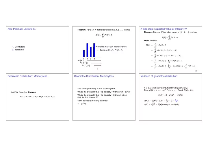
Theorem: For a r.v. X that takes values in {0,1,2,...}, one has E[X] =

∞

∑

i=1

Pr[X ≥ i]. 1 2 3 ··· Pr[X ≥ 1] Pr[X ≥ 2] Pr[X ≥ 3] . . . Probability mass at i, counted i times. Same as ∑∞

i=1 i ×Pr[X = i].

A side step: Expected Value of Integer RV

Theorem: For a r.v. X that takes values in {0,1,2,...}, one has E[X] =

∞

∑

i=1

Pr[X ≥ i]. Proof: One has

E[X] =

∞

∑

i=1

i ×Pr[X = i] =

∞

∑

i=1

i (Pr[X ≥ i]−Pr[X ≥ i +1]) =

∞

∑

i=1

(i ×Pr[X ≥ i]−i ×Pr[X ≥ i +1]) =

∞

∑

i=1

i ×Pr[X ≥ i]−

∞

∑

i=1

i ×Pr[X ≥ i +1] =

∞

∑

i=1

i ×Pr[X ≥ i]−

∞

∑

i=1

(i −1)×Pr[X ≥ i] =

∞

∑

i=1

Pr[X ≥ i].

Geometric Distribution: Memoryless

Let X be Geom(p). Theorem Pr[X > n +m|X > n] = Pr[X > m],m,n ≥ 0.

Geometric Distribution: Memoryless

I flip a coin (probability of H is p) until I get H. What’s the probability that I flip it exactly 100 times? (1−p)99p What’s the probability that I flip it exactly 100 times if (given that) the first 20 were T? Same as flipping it exactly 80 times! (1−p)79p.

Variance of geometric distribution.

X is a geometrically distributed RV with parameter p. Thus, Pr[X = n] = (1−p)n−1p for n ≥ 1. Recall E[X] = 1/p. E[X 2] = (2−p)/p2 (tricks) var[X] = E[X 2]−E[X]2 = 2−p

p2 − 1 p2 = 1−p p2 .

σ(X) = √

1−p p

≈ E[X] when p is small(ish).

SLIDE 2

Poisson

Experiment: flip a coin n times. The coin is such that Pr[H] = λ/n. Random Variable: X - number of heads. Thus, X = B(n,λ/n). Poisson Distribution is distribution of X “for large n.”

Poisson

Experiment: flip a coin n times. The coin is such that Pr[H] = λ/n. Random Variable: X - number of heads. Thus, X = B(n,λ/n). Poisson Distribution is distribution of X “for large n.”

We expect X ≪ n. For m ≪ n one has Pr[X = m] = λ m m! e−λ.

Poisson Distribution: Definition and Mean

Definition Poisson Distribution with parameter λ > 0 X = P(λ) ⇔ Pr[X = m] = λ m m! e−λ,m ≥ 0. Fact: E[X] = λ.

Poisson and Queueing.

Poisson: Distribution of how many events in an interval? Average: λ. What is the maximum number of customers you might see? Idea: Cut into intervals so that “sum of Bernoulli (indicators)”. n = 10 sub-intervals. Binomial distribution, if only one event/interval! Maybe more... and more. As n goes to infinity...analyze ... .... Pr[X = i] = n

i

• pi(1−p)n−i.

derive simple expression. ...And we get the Poisson distribution!

When to use Poisson

If an event can occur 0,1,2,... times in an interval, and the average number of events per interval is λ and events are independent and the probability of an event in an interval is proportional to the interval’s length, then it might be appropriate to use Poisson distribution. Pr[k events in interval] = λ k k! e−λ Examples: photons arriving at a telescope, telephone calls arriving in a system, the number of mutations on a strand of DNA per unit length...

Simeon Poisson

The Poisson distribution is named after: “Life is good for only two things: doing mathematics and teaching it.”

SLIDE 3

Review: Distributions

◮ Bern(p) : Pr[X = 1] = p;

E[X] = p; Var[X] = p(1−p);

◮ B(n,p) : Pr[X = m] =

n

m

• pm(1−p)n−m,m = 0,...,n;

E[X] = np; Var[X] = np(1−p);

◮ U[1,...,n] : Pr[X = m] = 1 n,m = 1,...,n;

E[X] = n+1

2 ;

Var[X] = n2−1

12 ; ◮ Geom(p) : Pr[X = n] = (1−p)n−1p,n = 1,2,...;

E[X] = 1

p;

Var[X] = 1−p

p2 ; ◮ P(λ) : Pr[X = n] = λ n n! e−λ,n ≥ 0;

E[X] = λ; Var[X] = λ.

Inequalities: An Overview

n p n

µ P r [|X − µ | > ]

• Chebyshev

n p n

p n

Distribution

n p n

P r [X > a ] a Markov µ

Andrey Markov

Andrey Markov is best known for his work on stochastic processes. A primary subject of his research later became known as Markov chains and Markov processes. Pafnuty Chebyshev was one of his teachers.

Markov’s inequality

The inequality is named after Andrey Markov, although it appeared earlier in the work of Pafnuty Chebyshev. It should be (and is sometimes) called Chebyshev’s first inequality.

Theorem Markov’s Inequality (the fancy version) Assume f : ℜ → [0,∞) is nondecreasing. Then, for a non-negative random variable X Pr[X ≥ a] ≤ E[f(X)] f(a) , for all a such that f(a) > 0. Proof: Observe that 1{X ≥ a} ≤ f(X) f(a) . Indeed, if X < a, the inequality reads 0 ≤ f(X)/f(a), which holds since f(·) ≥ 0. Also, if X ≥ a, it reads 1 ≤ f(X)/f(a), which holds since f(·) is nondecreasing. Expectation is monotone: if X(ω) ≤ Y(ω) for all ω, then E[X] ≤ E[Y]. Therefore, E[1{X ≥ a}] ≤ E[f(X)] f(a) .

A picture Markov Inequality Note

A more common version of Markov is for f(x) = x: Theorem For a non-negative random variable X, and any a > 0, Pr[X ≥ a] ≤ E[X] a .

SLIDE 4

Markov Inequality Example: Geom(p)

Let X ∼ Geom(p). Recall that E[X] = 1

p and E[X 2] = 2−p p2 .

Choosing f(x) = x, we get Pr[X ≥ a] ≤ E[X] a = 1 ap . Choosing f(x) = x2, we get Pr[X ≥ a] ≤ E[X 2] a2 = 2−p p2a2 .

Markov’s inequality example

Pr[X ≥ a] ≤ E[X] a . What is a bound on the probability that a random X takes value ≥ than twice its’ expectation?

1

• 2. It can’t be that more than half of the people are twice above

the average! What is a bound on the probability that a random X takes value ≥ than k times its’ expectation?

1 k .

Markov’s inequality example

Flip a coin n times. Probability of H is p. X counts the number

• f heads.

X follows the Binomial distribution with parameters n and p. X ∼ B(n,p). E[X] = np. Say n = 1000 and p = 0.5. E[X] = 500. Markov says that Pr[X ≥ 600] ≤ 1000∗0.5

600

= 5

6 ≈ 0.83

Actual probability: < 0.000001 Notice: Same bound for 10 coins and Pr[X ≥ 6]

Chebyshev’s Inequality

This is Pafnuty’s inequality: Theorem: Pr[|X −E[X]| ≥ a] ≤ var[X] a2 , for all a > 0. Proof: Let Y = |X −E[X]| and f(y) = y2. Then, Pr[Y ≥ a] ≤ E[f(Y)] f(a) = E[|X −E[X]|2] a2 = var[X] a2 . This result confirms that the variance measures the “deviations from the mean.”

Chebyshev and Poisson

Let X = P(λ). Then, E[X] = λ and var[X] = λ. Thus, Pr[|X −λ| ≥ n] ≤ var[X] n2 = λ n2 .

Chebyshev’s inequality example

Flip a coin n times. Probability of H is p. X counts the number

• f heads.

X follows the Binomial distribution with parameters n and p. X ∼ B(n,p). E[X] = np. Var[X] = np(1−p). Say n = 1000 and p = 0.5. E[X] = 500. Var[X] = 250. Markov says that Pr[X ≥ 600] ≤ 500

600 = 5 6 ≈ 0.83

Chebyshev says that Pr[X ≥ 600] = Pr[X −500 ≥ 100] ≤ Pr[|X −500| ≥ 100] ≤

250 10000 = 0.025

Actual probability: < 0.000001 Notice: If we had 100 coins, the bound for Pr[X ≥ 60] would be different.

SLIDE 5

Chebyshev’s inequality example continued

What if we had more coins? Also, let’s count the fraction of H instead of their number. p is still 0.5 Let Xi be the indicator random variable for the i-th coin. Define Yn = X1 +···+Xn n , for n ≥ 1. E[Yn] = 1

nE[∑Xi] = 1 nnp = p = 0.5

Var[Yn] = 1

n2 Var[∑Xi] = 1 n2 np(1−p) = p(1−p) n

= 1

4n

Let’s try to bound how likely it is that the fraction of H’s differs from 50%. Pr[|Yn −0.5| ≥ ε]?

Chebyshev’s inequality example continued

E[Yn] = 0.5, Var[Yn] = 1

4n.

Pr[|Yn −0.5| ≥ ε] ≤ Var[Yn] ε2 = 1 4nε2 For ε = 0.01: Pr[|Yn −0.5| ≥ 0.01] ≤ 2500

n

For n = 250,000 this is 1%. As n → ∞, this probability goes to zero. In fact, for any ε > 0, as n → ∞, the probability that the fraction

• f Hs is within ε > 0 of 50% approaches 1:

Pr[|Yn −0.5| ≤ ε] → 1. This is an example of the Law of Large Numbers. We look at a general case next.

Weak Law of Large Numbers

Theorem Weak Law of Large Numbers Let X1,X2,... be pairwise independent with the same distribution and mean µ. Then, for all ε > 0, Pr[|X1 +···+Xn n − µ| ≥ ε] → 0, as n → ∞. Proof: Let Yn = X1+···+Xn

n

. Then Pr[|Yn − µ| ≥ ε] ≤ var[Yn] ε2 = var[X1 +···+Xn] n2ε2 = nvar[X1] n2ε2 = var[X1] nε2 → 0, as n → ∞. (I used that variance is finite for this proof. More complicated proof without this assumption.)

Confidence intervals example

Say p in the previous example was unknown. If you flip n coins, your estimate for p is ˆ p = 1

n ∑n i=1 Xi.

You many coins do you have to flip to make sure that your estimation ˆ p is within 0.01 of the true p, with probability at least 95%? E[ˆ p] = E[ 1

n ∑n i=1 Xi] = p

Var[ˆ p] = Var[ 1

n ∑n i=1 Xi] = 1 n2 Var[∑n i=1 Xi] = p(1−p) n

Pr[|ˆ p −p| ≥ ε] ≤ Var[ˆ p] ε2 = p(1−p) nε2

Confidence intervals example continued

Estimation ˆ p is within 0.01 of the true p, with probability at least 95%. Pr[|ˆ p −p| ≥ ε] ≤ p(1−p) nε2 We want to make Pr[|ˆ p −p| ≤ 0.01] at least 0.95. Same as Pr[|ˆ p −p| ≥ 0.01] at most 0.05. It’s sufficient to have p(1−p)

nε2

≤ 0.05 or n ≥ 20p(1−p)

ε2

. p(1−p) is maximized for p = 0.5. Therefore it’s sufficient to have n ≥ 5

ε2 .

For ε = 0.01 we get that n ≥ 50000 coins are sufficient.

Today’s gig: ?

Gigs so far:

• 1. How to tell random from human.
• 2. Monty Hall.
• 3. Birthday Paradox.
• 4. St. Petersburg paradox.
• 5. Simpson’s paradox.
• 6. Two envelopes problem.

Today: A magic trick.

SLIDE 6

Summary

◮ Variance of Geometric. ◮ Markov’s Inequality ◮ Chebyshev’s Inequality.