
SLIDE 1
Planning and Optimization
- G8. Monte-Carlo Tree Search Algorithms (Part II)
Malte Helmert and Thomas Keller
Universit¨ at Basel
December 16, 2019
- M. Helmert, T. Keller (Universit¨
at Basel) Planning and Optimization December 16, 2019 1 / 25
Planning and Optimization
December 16, 2019 — G8. Monte-Carlo Tree Search Algorithms (Part II)
G8.1 ε-greedy G8.2 Softmax G8.3 UCB1 G8.4 Summary
- M. Helmert, T. Keller (Universit¨
at Basel) Planning and Optimization December 16, 2019 2 / 25
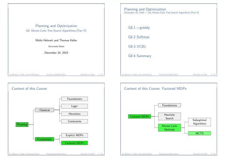
Content of this Course
Planning Classical Foundations Logic Heuristics Constraints Probabilistic Explicit MDPs Factored MDPs
- M. Helmert, T. Keller (Universit¨
at Basel) Planning and Optimization December 16, 2019 3 / 25
Content of this Course: Factored MDPs
Factored MDPs Foundations Heuristic Search Monte-Carlo Methods Suboptimal Algorithms MCTS
- M. Helmert, T. Keller (Universit¨
at Basel) Planning and Optimization December 16, 2019 4 / 25