parsing beyond context free grammar
play

Parsing beyond context-free grammar: S ( 0 , n ) for any w T - PowerPoint PPT Presentation

Kallmeyer/Maier Sommersemester 2009 Kallmeyer/Maier Sommersemester 2009 Elimination of useless rules (1) Boullier (1998) A useless rule is a rule which cannot be used in a derivation Parsing beyond context-free grammar: S ( 0 , n


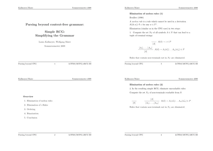
  1. Kallmeyer/Maier Sommersemester 2009 Kallmeyer/Maier Sommersemester 2009 Elimination of useless rules (1) Boullier (1998) A useless rule is a rule which cannot be used in a derivation Parsing beyond context-free grammar: ∗ S ( � 0 , n � ) ⇒ ε for any w ∈ T ∗ . Elimination (similar as in the CFG case) in two steps: Simple RCG: 1. Compute the set N T of all symbols A ∈ N that can lead to a Simplifying the Grammar tuple of terminal strings: A ( � α ) → ε ∈ P Laura Kallmeyer, Wolfgang Maier [ A ] Sommersemester 2009 [ A 1 ] , . . ., [ A m ] α ) → A 1 ( � α m ) ∈ P A ( � α 1 ) . . . A m ( � [ A ] Rules that contain non-terminals not in N T are eliminated. Parsing beyond CFG 1 LCFRS/MCFG/sRCG III Parsing beyond CFG 3 LCFRS/MCFG/sRCG III Kallmeyer/Maier Sommersemester 2009 Kallmeyer/Maier Sommersemester 2009 Elimination of useless rules (2) 2. In the resulting simple RCG, eliminate unreachable rules: Compute the set N S of non-terminals reachable from S : Overview [ A ] 1. Elimination of useless rules A ( � α ) → A 1 ( � α 1 ) . . .A m ( � α m ) ∈ P [ S ] [ A 1 ] , . . ., [ A m ] 2. Elimination of ε -Rules Rules that contain non-terminals not in N S are eliminated. 3. Ordering 4. Binarization 5. Conclusion Parsing beyond CFG 2 LCFRS/MCFG/sRCG III Parsing beyond CFG 4 LCFRS/MCFG/sRCG III
  2. Kallmeyer/Maier Sommersemester 2009 Kallmeyer/Maier Sommersemester 2009 Elimination of ε -Rules (1) Elimination of ε -Rules (3) An ε -rule is a rule with one of the lhs arguments being ε . The set N ǫ is constructed recursively with initial value ∅ : 1. For every A ( x 1 , . . ., x k ) → ǫ ∈ P : A simple RCG is ǫ -free if ι ) to N ǫ with for all 1 ≤ i ≤ k : � Add ( A,� ι ( i ) = 0 if x i = ε , else • it either contains no ǫ -rules ι ( i ) = 1 for all 1 ≤ i ≤ k . � • or there is exactly one rule S ( ǫ ) → ǫ and S does not appear in 2. Repeat until N ǫ does not change any more: any rhs of a rule in G For every A ( x 1 , . . ., x k ) → A 1 ( α 1 ) . . .A m ( α m ) and all ( A 1 ,� ι 1 ), . . . , ( A m ,� ι m ) ∈ N ǫ : • Calculate a vector ( x ′ 1 , . . ., x ′ k ) from ( x 1 , . . ., x k ) by removing every variable that is the j th variable of A i in the righthand side such that � ι i ( j ) = 0 with ε . • Then add ( A,� ι ) to N ǫ with for all 1 ≤ i ≤ k : � ι ( i ) = 0 if x ′ i = ǫ , else � ι ( i ) = 1. Parsing beyond CFG 5 LCFRS/MCFG/sRCG III Parsing beyond CFG 7 LCFRS/MCFG/sRCG III Kallmeyer/Maier Sommersemester 2009 Kallmeyer/Maier Sommersemester 2009 Elimination of ε -Rules (2) Elimination of ε -Rules (4) Now we can compute the new set of rules: First, compute for all A ∈ N , all possibilities to have ε -components in their yields: For every clause A ( x 1 , . . ., x k ) → A 1 ( x (1) 1 , . . ., x (1) k 1 ) . . .A m ( x ( m ) , . . ., x ( m ) k m ) and all ι ∈ { 0 , 1 } dim ( A ) , and • We introduce vectors � 1 ( A 1 ,� ι 1 ), . . . , ( A m ,� ι m ) ∈ N ǫ , we compute a clause for the new • we compute the set N ε of pairs ( A,� ι ) where � ι signifies that it is grammar: possible for A to have a tuple τ in its yield with τ ( i ) = ε if • In the rhs, we replace A i with ( A i ,� ι i ) for all 1 ≤ i ≤ m ; � ι ( i ) = 0 and τ ( i ) � = ε if � ι ( i ) � = 0. • in both, lhs and rhs, we delete all variables x ( i ) for 1 ≤ i ≤ m j and 1 ≤ j ≤ k i with � ι i ( j ) = 0; • in the lhs, we replace A with ( A,� ι ) where � ι ( l ) = 0 iff the i th argument is ε ; • finally delete all ε -arguments in lhs and rhs. Furthermore, we add a new start symbol ( S ′ ) with S ′ ( X ) → S 1 ( X ) and, if ε in the language, S ′ ( ε ) → ε . Parsing beyond CFG 6 LCFRS/MCFG/sRCG III Parsing beyond CFG 8 LCFRS/MCFG/sRCG III

  3. Kallmeyer/Maier Sommersemester 2009 Kallmeyer/Maier Sommersemester 2009 Elimination of ε -Rules (5) Ordered simple RCG (2) Transformation into an ordered simple RCG: Example: Original simple RCG rules: P ′ := P ; S ( XY ) → A ( X, Y ), A ( a, ε ) → ε , A ( ε, a ) → ε , A ( a, b ) → ε repeat until P ′ does not change any more: Set of pairs characterizing possibilities for ε -components: for all rules r = A ( � α ) → A 1 ( � α 1 ) . . . A k ( � α k ) in P ′ : for all i , 1 ≤ i ≤ k : N ε = { ( S, 1) , ( A, 10) , ( A, 01) , ( A, 11) } if A i ( � α i ) = A i ( Y 1 , . . . , Y dim ( A i ) ) and Rules after ε -elimination: the order of the Y 1 , . . . , Y dim ( A i ) in � α is S ′ ( X ) → S 1 ( X ), p ( Y 1 , . . . , Y dim ( A i ) ) where p is not the identity S 1 ( X ) → A 10 ( X ), A 10 ( a ) → ε , then α i ) in r with A p replace A i ( � i ( p ( � α i )) ; S 1 ( X ) → A 01 ( X ), A 01 ( b ) → ε , for every A i -rule A i ( � γ ) → Γ ∈ P ′ : S 1 ( XY ) → A 11 ( X, Y ), A 11 ( a, b ) → ε add a new rule A p i ( p ( � γ )) → Γ to P ′ (if not yet in P ′ ) Parsing beyond CFG 9 LCFRS/MCFG/sRCG III Parsing beyond CFG 11 LCFRS/MCFG/sRCG III Kallmeyer/Maier Sommersemester 2009 Kallmeyer/Maier Sommersemester 2009 Ordered simple RCG (1) Ordered simple RCG (3) A simple RCG is ordered if for every rule Example: A ( � α ) → A 1 ( � α 1 ) . . .A k ( � α k ) Original clauses: S ( XY ) → A ( X, Y ), A ( X, Y ) → A ( Y, X ), A ( aX, bY ) → A ( X, Y ), and every A i ( � α i ) = A i ( Y 1 , . . ., Y dim ( A i ) ) (1 ≤ i ≤ k ), the order of A ( a, b ) → ε the components of � α i in � α is Y 1 , . . ., Y dim ( A i ) . Clauses after transformation into ordered RCG: Crucially, in an ordered simple RCG, the order of the components S ( XY ) → A ( X, Y ), A ( X, Y ) → A p ( X, Y ), A ( aX, bY ) → A ( X, Y ), of the lhs predicate of a rule corresponds always to their order in A ( a, b ) → ε , A p ( Y, X ) → A ( Y, X ), A p ( bY, aX ) → A p ( Y, X ), the input. A p ( b, a ) → ε ( p being the permutation that switches the two arguments) For every simple RCG, there exists a weakly equivalent ordered simple RCG. For the transformation, in addition to the A ∈ N , we introduce new predicates A p where p a permutation of � 1 , . . ., dim ( A ) � . Parsing beyond CFG 10 LCFRS/MCFG/sRCG III Parsing beyond CFG 12 LCFRS/MCFG/sRCG III

  4. Kallmeyer/Maier Sommersemester 2009 Kallmeyer/Maier Sommersemester 2009 Binarization (1) Binarization (3) Binarization algorithm: We call the length of the rhs of a rule its rank . The rank of a simple RCG is given by the maximal rank of its rules. α ) → A 0 ( � for all rules r = A ( � α 0 ) . . . A m ( � α m ) in P with m > 1 : remove r from P ; For every simple RCG, there is an equivalent simple RCG of rank 2. R := ∅ ; CNF binarization for CFG: A → BCD replaced with A → BE , pick new predicate names C 1 , . . . , C m − 1 ; E → CD add A ( � α ) → A 0 ( � α 0 ) C 1 ( � γ 1 ) to R where � γ 1 is � α reduced with � α 0 ; A similar binarization algorithm can be applied to LCFRS/simple for all i , 1 ≤ i < m − 1 : RCG: add C i ( � γ i ) → A i ( � α i ) C i +1 ( � γ i +1 ) to R where For every rule with rhs length > 2, we introduce a new predicate γ i +1 is � � γ i reduced with � α i ; that comprises all rhs predicates except the first. This is done add C m − 1 ( γ m − 2 ) → A m − 1 ( α m − 1 ) A m ( � α m ) to R ; � � repeatedly. for every r ′ ∈ R : replace rhs arguments of length > 1 with new variables (in both sides) and add the result to P Parsing beyond CFG 13 LCFRS/MCFG/sRCG III Parsing beyond CFG 15 LCFRS/MCFG/sRCG III Kallmeyer/Maier Sommersemester 2009 Kallmeyer/Maier Sommersemester 2009 Binarization (2) Binarization (4) α 1 ∈ [( T ∪ V ) ∗ ] k 1 by We define the reduction of a � Example: Original simple RCG: � X 1 , . . ., X k 2 � ∈ V k 2 where all X i for 1 ≤ i ≤ k 2 occur in � α 1 as the S ( XY ZUV W ) → A ( X, U ) B ( Y, V ) C ( Z, W ) following vector of variables: A ( aX, aY ) → A ( X, Y ) B ( bX, bY ) → B ( X, Y ) C ( cX, cY ) → C ( X, Y ) We take all variables from � α 1 (in their order) that are not in A ( a, a ) → ε B ( b, b ) → ε C ( c, c ) → ε { X 1 , . . ., X k 2 } while starting a new component whenever a variable is, in � α 1 , in a different component than the preceding variable in For the rule with righthand side of length > 2 we obtain the result or in the same component but not adjacent to it. R = { S ( XY ZUV W ) → A ( X, U ) C 1 ( Y Z, V W ), C 1 ( Y Z, V W ) → B ( Y, V ) C ( Z, W ) } Examples: 1. � aX 1 , X 2 , bX 3 � reduced with � X 2 � yields � X 1 , X 3 � ; Equivalent simple RCG of rank 2: S ( XPUQ ) → A ( X, U ) C 1 ( P, Q ) C 1 ( Y Z, V W ) → B ( Y, V ) C ( Z, W ) 2. � aX 1 X 2 bX 3 � reduced with � X 2 � yields � X 1 , X 3 � . A ( aX, aY ) → A ( X, Y ) B ( bX, bY ) → B ( X, Y ) C ( cX, cY ) → C ( X, Y ) A ( a, a ) → ε B ( b, b ) → ε C ( c, c ) → ε Parsing beyond CFG 14 LCFRS/MCFG/sRCG III Parsing beyond CFG 16 LCFRS/MCFG/sRCG III

Download Presentation
Download Policy: The content available on the website is offered to you 'AS IS' for your personal information and use only. It cannot be commercialized, licensed, or distributed on other websites without prior consent from the author. To download a presentation, simply click this link. If you encounter any difficulties during the download process, it's possible that the publisher has removed the file from their server.

Recommend


More recommend