Parallel Numerical Algorithms Solution of Boundary Value Problems 1 - PowerPoint PPT Presentation
Parallel Numerical Algorithms Solution of Boundary Value Problems 1 Overview of Lecture General solution methods Relaxation methods Jacobi algorithm testing for convergence Gauss Seidel over-relaxation Notes
Parallel Numerical Algorithms Solution of Boundary Value Problems 1
Overview of Lecture General solution methods Relaxation methods – Jacobi algorithm – testing for convergence – Gauss Seidel – over-relaxation Notes – parallelisation – non-linear equations Pollution problem – solution using relaxation methods – 2D equations including wind 2
Many methods for solving Au = b Direct methods – give the solution after a fixed number of operations • Gaussian elimination • LU factorisation Relaxation methods (this lecture) – gradually improve solution, starting from an initial guess – stop when the answer is sufficiently accurate – simple to implement but may be slow to converge on solution • or may fail completely! Krylov subspace methods (following lectures) – iterative (like relaxation methods) but more sophisticated – harder to implement but more efficient and reliable 3
Why not use Direct Methods? Direct methods explicitly operate on the matrix A – eg decompose it into L and U factors For PDEs, A is very sparse indeed – may contain 99% zeros so clearly we use compressed storage – we want to take advantage of this when we solve equations Difficult to exploit sparsity for direct methods – eg L and U may be dense even though A is sparse – for large systems of equations, we may run out of memory! Relaxation and Krylov methods exploit sparsity – relaxation methods operate on the equations not the matrix – Krylov methods comprise mostly matrix-vector multiplications • can write efficient routines to do y = A x when A is sparse 4
Relaxation vs Matrix Methods Operate directly on the difference equations – can forget (almost!) all about the matrix representation Au = b for this lecture – it turns out that relaxation methods can usefully be understood in terms of matrix-vector operations (not immediately obvious) • See lecture on “Matrix Splitting Techniques” For illustrative purposes, look at 1D problem – for simplicity with no wind – exercise will involve extending this to the 2D problem • quite straightforward in practice 5
Relaxation Methods 1D diffusion equations are - u i -1 + 2 u i - u i+ 1 = 0, i = 1, 2, ... N Equivalently: u i = ½ ( u i -1 + u i+ 1 ) – why not make an initial guess at the solution – then loop over each lattice point i and set u i = ½ ( u i -1 + u i+ 1 ) – ie we solve the equation exactly at each point in turn Updating u i spoils solution we just did for u i-1 – so simply iterate the whole process again and again ... – ... and hope we eventually get the right answer! This is called the Jacobi Algorithm – the simplest possible relaxation method 6
Jacobi Algorithm Use superscript n to indicate iteration number – n counts the number of times we update the whole solution – equivalent to computer time Jacobi algorithm for diffusion equation is: ( n +1) = ½ ( u i-1 ( n ) + u i+1 ( n ) ) u i Each iteration, calculate u ( n+1 ) in terms of u ( n ) – don’t need to keep copies of all the previous solutions – only need to remember two solutions at any time: u and u new • corresponding to iterations n and n +1 7
Jacobi Pseudo-Code declare arrays : u(0, 1, ..., M+1) unew(0, 1, ..., M+1) initialise : set boundaries : u(0) = fixed value u 0 u(M+1) = fixed value u M+1 initial guess : u(1, 2, ..., M) = guess value loop over n = 1, 2, ... update : loop over internal points: i = 1, 2, ... M unew(i) = 0.5*( u(i-1) + u(i+1) ) end loop over i copy back : u(1, 2, ..., M) = unew(1, 2, ..., M) end loop over n 8
Implementation Notes Array declarations – Fortran: real, dimension(0:M+1) :: u – Java: float[] u = new float[M+2]; – C: float u[M+2]; Arrays explicitly contain boundaries u 0 and u M +1 – we set them according to boundary conditions • but we NEVER update them! – eg when we copy u new back to u , only copy internal values – in pseudo-code, boundary values for u new are never set • complete solution is therefore only ever present in u • might be more elegant to set boundaries in u new as well What to choose for initial guess u i (0) ? – for a simple implementation just set interior values to zero 9
Progress of Solution n= 1 n = 0 6 6 5 5 4 4 3 3 2 2 1 1 0 0 1 2 3 4 5 6 7 8 9 0 -1 0 1 2 3 4 5 6 7 8 9 -1 n = 20 n = 5 6 6 5 5 4 4 3 3 2 2 1 1 0 0 0 1 2 3 4 5 6 7 8 9 0 1 2 3 4 5 6 7 8 9 -1 -1 10
When to Stop the Iterative Loop The solution appears to be getting better – must quantify this! For dense systems we used the residual – we tried to solve Ax = b , so r = b-Ax should be a zero vector – in practice, there is a numerical error in solution of each equation – error in equation i is the value of r i • residual is computed from the sum of the squares of r i Can do the same thing for relaxation methods – compute the sum of the squares of the error in each equation – do this at the end of each iterative loop over n • stop if this is small enough 11
Pseudocode for Residual Calculation loop over n = 1, 2, ... update : ... copy back : ... compute residue : rnorm = 0.0 loop over i = 1, 2, ..., M rnorm = rnorm + (-u(i-1)+2*u(i)-u(i+1)) 2 end loop over n rnorm = sqrt(rnorm) normalise : res = rnorm / bnorm if (res < tolerance) finish end loop over n 12
Notes on Residual For a perfect solution, residue will be zero – in practice we will get a finite value – usually stop when it is “small”, eg a tolerance of res < 10 -6 – there will be a limit to how small the residual can get • can easily hit the limits of single precision • use double precision everywhere (or at least perform residual calculation using doubles) Normalisation – need to divide by the norm of the b vector – we saw before that b corresponds to the boundary values – in 1D: bnorm = sqrt(u(0)*u(0) + u(M+1)*u(M+1)) • in 2D, need to sum values of squares of u i,j over all edges 13
Residual Against Iteration 1.0E+00 1.0E-01 1.0E-02 1.0E-03 1.0E-04 0 20 40 60 80 100 Decreases exponentially – with a zero initial guess for u , should equal 1.0 at iteration zero 14
Parallelisation Very simple for Jacobi Decompose the problem domain regularly across processes/threads – for MPI we need halo regions due to i +1, i -1 references – halos are 1 cell wide for 5-point stencil – could be wider for larger stencils – swap halos between neighbouring processes every iteration Require global sums for, eg, residue calculation 15
Relaxation Methods About to cover some variations on Jacobi – which we hope will be faster! How can we tell if a method will work at all? Necessary (but not sufficient) condition – if the method arrives at the correct solution it must stay there Is this true for Jacobi? ( n +1) = ½ ( u i-1 ( n ) + u i+1 ( n ) ) u i – for a solution: - u i -1 ( n ) +2 u i ( n ) - u i+ 1 ( n ) = 0, ie ½ ( u i -1 ( n ) ( n ) ) = u i ( n ) + u i+ 1 – so, u i ( n +1) = u i ( n ) and we stay at the solution • worth checking this for other methods 16
Gauss Seidel Why do we need both u new and u ? update : loop over internal points: i = 1, 2, ... M unew(i) = 0.5*( u(i-1) + u(i+1) ) end loop over i copy back : u(1, 2, ..., M) = unew(1, 2, ..., M) Why not do the update in place? update : loop over internal points: i = 1, 2, ... M u(i) = 0.5*( u(i-1) + u(i+1) ) end loop over i – this is called the Gauss-Seidel method 17
Convergence of Gauss-Seidel 1.0E+00 1.0E-01 1.0E-02 1.0E-03 1.0E-04 1.0E-05 1.0E-06 1.0E-07 1.0E-08 0 20 40 60 80 100 Converges twice as fast as Jacobi – for less work and less storage! 18
Notes on Gauss Seidel Order of the update loop is now significant – we used normal ( lexicographic ) order: other orderings possible Red-black order divides grid into chequerboard – update all the red squares first then all the black ones – enables Gauss Seidel method to be parallelised Processor 1 Processor 2 19
Over Relaxation Recall how Jacobi solution progressed ( n ) u i +1 ( n +1) u i ( n ) u i ( n ) u i -1 – we have increased the value of u i by a small amount • but we know the real solution is even higher – why not increase by more than suggested • ie multiply the change by some factor w > 1 20
Over-Relaxed Gauss Seidel Gauss-Seidel method: u i = ½ ( u i-1 + u i+1 ) – ie: u i = u i + [ ½ ( u i-1 – 2 u i + u i+1 ) ] Multiply change (in square brackets) by w – over-relaxed update: u i = u i + ½ w ( u i-1 – 2 u i + u i+1 ) – or u i = (1- w ) u i + ½ w ( u i-1 + u i+1 ) Notes – original method corresponds to w = 1 – if we get to a solution we stay there for any value of w 21
Non-Linear Equations Relaxation methods deal directly with equations – doesn’t matter that we cannot express them as Au = b – equally valid for non-linear equations (eg fluid dynamics) Non-linear equations can be very unstable – may need to under-relax to get convergence, ie w < 1 22
Recommend
More recommend
Explore More Topics
Stay informed with curated content and fresh updates.
