
SLIDE 1
Matrix multiplication
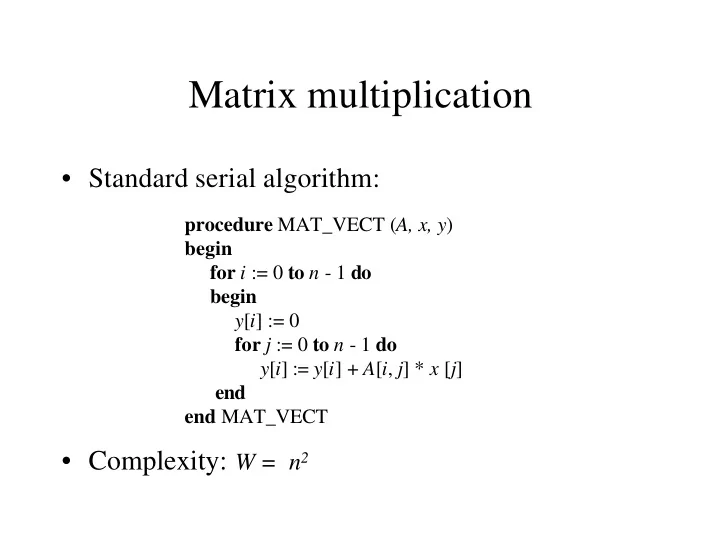
- Standard serial algorithm:
- Complexity: W = n2
Matrix multiplication Standard serial algorithm: procedure MAT_VECT - - PowerPoint PPT Presentation
Matrix multiplication Standard serial algorithm: procedure MAT_VECT ( A, x, y ) begin for i := 0 to n - 1 do begin y [ i ] := 0 for j := 0 to n - 1 do y [ i ] := y [ i ] + A [ i , j ] * x [ j ] end end MAT_VECT Complexity: W = n 2
– A2A broadcast of vector elements: Θ(n) – single row multiplication: Θ(n) – Total time: Θ(n) – processor-time product: Θ(n2) (cost-opt.)
– A2A broadcast of vector elements:
(mesh)
– row multiplication: Θ(n2/p) – total time:
(mesh)
– one-to-one comm. + one-2-all broadcast + single node accumul. per row + multipl. = = Θ(n) + Θ(n) + Θ(n) + Θ(1) = Θ(n) (mesh) = Θ(log n) + Θ(log n) + … = Θ(log n) (hyper) – processor-time product:
(mesh)
– each processor stores a (n√p × n√p) block – Run time on mesh with CT: – Θ(n/√p) + Θ((n/√p) log p) + Θ((n/√p) log p) + Θ(n2/p) – Cost optimal as long as p = O (n2/log2n )
– q3 matrix multiplications each involving n/q × n/q elements and requiring (n/q)3 multiplications and additions procedure BLOCK_MAT_MULT(A, B, C) begin for i := 0 to q - 1 do for j := 0 to q - 1 do begin Initialize all elements of Ci,j to zero for k := 0 to q - 1 do Ci,j := Ci, j + Ai, k * Bk, j end end BLOCK_MAT_MULT
–
, Pi, j needs all blocks Ai, k and Bk, j for 0 ≤ k ≤ √p, thus an A2A
a0,0x0 + a0,1x1 + … + a0,n-1xn-1 = b0 a1,0x0 + a1,1x1 + … + a1,n-1xn-1 = b1 . . . . . . . . . . . . an-1,0x0 + an-1,1x1 + … + an-1,n-1xn-1 = bn-1 x0 + u0,1x1 + … + u0,n-1xn-1 = y0 x1 + … + u1,n-1xn-1 = y1 . . . . . . xn-1 = yn-1
Gaussian elimination
– kth computation step: 3(n-k-1) – Total computation: 3n(n-1)/2 – kth comm. step: (ts + tw(n-k-1))logn (on hypercube) – Tot. comm. : (tsn + twn(n-1)/2)logn – Cost: Θ(n3 logn)
– row k+1 can start computation as soon as it gets data from row k – this optimized version of the alg. is cost-
– block-striped partitioning
hypercube)
processors are idle
– cyclic-striped partitioning
– system is discretized by superimposing grid – temperature at each point is computed based on neighbor values