Papers Covered Change Blindness Change Blindness Current - - PowerPoint PPT Presentation

SLIDE 1

Perception

CS533C Presentation by Alex Gukov

Papers Covered



Current approaches to change blindness Daniel J. Simons. Visual Cognition 7, 1/2/3 (2000)



Internal vs. External Information in Visual Perception Ronald

• A. Rensink. Proc. 2nd Int. Symposium on Smart Graphics,

pp 63-70, 2002



Visualizing Data with Motion Daniel E. Huber and Christopher G. Healey. Proc. IEEE Visualization 2005, pp. 527-534.



Stevens Dot Patterns for 2D Flow Visualization. Laura G. Tateosian, Brent M. Dennis, and Christopher G. Healey.

• Proc. Applied Perception in Graphics and Visualization

(APGV) 2006

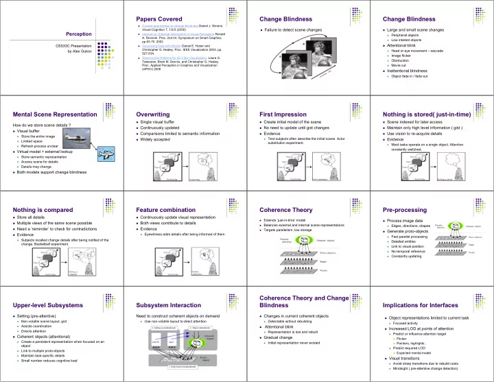
Change Blindness

 Failure to detect scene changes

Change Blindness

 Large and small scene changes

 Peripheral objects  Low interest objects

 Attentional blink

 Head or eye movement – saccade  Image flicker  Obstruction  Movie cut

 Inattentional blindness

 Object fade in / fade out

Mental Scene Representation

How do we store scene details ?

 Visual buffer

 Store the entire image  Limited space  Refresh process unclear

 Virtual model + external lookup

 Store semantic representation  Access scene for details  Details may change

 Both models support change blindness

Overwriting

 Single visual buffer  Continuously updated  Comparisons limited to semantic information  Widely accepted

First Impression

 Create initial model of the scene  No need to update until gist changes  Evidence

 Test subjects often describe the initial scene. Actor

substitution experiment.

Nothing is stored( just-in-time)

 Scene indexed for later access  Maintain only high level information ( gist )  Use vision to re-acquire details  Evidence

 Most tasks operate on a single object. Attention

constantly switched.

Nothing is compared

 Store all details  Multiple views of the same scene possible  Need a ‘reminder’ to check for contradictions  Evidence

 Subjects recalled change details after being notified of the

• change. Basketball experiment.

Feature combination

 Continuously update visual representation  Both views contribute to details  Evidence

 Eyewitness adds details after being informed of them.

Coherence Theory

 Extends ‘just-in-time’ model  Balances external and internal scene representations  Targets parallelism, low storage

Pre-processing

 Process image data

 Edges, directions, shapes

 Generate proto-objects

 Fast parallel processing  Detailed entities  Link to visual position  No temporal reference  Constantly updating

Upper-level Subsystems

 Setting (pre-attentive)

 Non-volatile scene layout, gist  Assists coordination  Directs attention

 Coherent objects (attentional)

 Create a persistent representation when focused on an

• bject

 Link to multiple proto-objects  Maintain task-specific details  Small number reduces cognitive load

Subsystem Interaction

Need to construct coherent objects on demand

 Use non-volatile layout to direct attention

Coherence Theory and Change Blindness

 Changes in current coherent objects

 Detectable without rebuilding

 Attentional blink

 Representation is lost and rebuilt

 Gradual change

 Initial representation never existed

Implications for Interfaces

 Object representations limited to current task

 Focused activity

 Increased LOD at points of attention

 Predict or influence attention target  Flicker  Pointers, highlights..  Predict required LOD  Expected mental model

 Visual transitions

 Avoid sharp transitions due to rebuild costs  Mindsight ( pre-attentive change detection)

SLIDE 2

Critique

 Extremely important phenomenon

 Will help understand fundamental perception mechanisms

 Theories lack convincing evidence

 Experiments do not address a specific goal  Experiment results can be interpreted in favour of a

specific theory (Basketball case)

Visualizing Data with Motion

 Multidimensional data sets more common  Common visualization cues

 Color  Texture  Position  Shape

 Cues available from motion

 Flicker  Direction  Speed

Previous Work

 Detection

 2-5% frequency difference from background  1o/s speed difference from the background  20o direction difference from the background  Peripheral objects need greater separation

 Grouping

 Oscillation pattern – must be in phase

 Notification

 Motion encoding superior to color, shape change

Flicker Experiment

 Test detection against background flicker  Coherency

 In phase / out of phase with the background

 Cycle difference  Cycle length

Flicker Experiment - Results

 Coherency

 Out of phase trials detection error ~50%  Exception for short cycles - 120ms  Appeared in phase

 Cycle difference, cycle length (coherent trials)

 High detection results for all values

Direction Experiment

 Test detection against background motion  Absolute direction  Direction difference

Direction Experiment - Results

 Absolute direction

 Does not affect detection

 Direction difference

 15o minimum for low error rate and detection time  Further difference has little effect

Speed Experiment

 Test detection against background motion  Absolute speed  Speed difference

Speed Experiment - Results

 Absolute speed 

Does not affect detection

 Speed difference 

0.42o/s minimum for low error rate and detection time



Further difference has little effect

Applications

 Can be used to visualize flow fields

 Original data 2D slices of 3D particle positions over

time (x,y,t)

 Animate keyframes

Applications Critique

 Study

 Grid density may affect results  Multiple target directions

 Technique

 Temporal change increases cognitive load  Color may be hard to track over time  Difficult to focus on details

Stevens Model for 2D Flow Visualization Idea

 Initial Setup

 Start with a regular dot pattern  Apply global transformation  Superimpose two patterns

 Glass

 Resulting pattern identifies the global transform

 Stevens

 Individual dot pairs create perception of local

direction

 Multiple transforms can be detected

Stevens Model

 Predict perceived direction

for a neighbourhood of dots

 Enumerate line segments in a

small neighbourhood

 Calculate segment directions  Penalize long segments  Select the most common

direction

 Repeat for all neighbourhoods

Stevens Model

Segment weight

SLIDE 3

Stevens Model

 Ideal neighbourhood – empirical results

 6-7 dots per neighbourhood  Density 0.0085 dots / pixel

 Neighbourhood radius

 16.19 pixels

 Implications for visualization algorithm

 Multiple zoom levels required

2D Flow Visualization

 Stevens model estimates perceived direction  How can we use it to visualize flow fields ?

 Construct a dot neighbourhoods such that the

desired direction matches what is perceived

Algorithm

 Data 

2D slices of 3D particle positions over a period of time

 Algorithm 

Start with a regular grid



Calculate direction error around a single point

 Desired direction: keyframe data  Perceived direction: Stevens model 

Move one of the neighbourhood points to decrease error



Repeat for all neighbourhoods

Results Critique

 Model



Shouldn’t we penalize segments which are too short ?

 Algorithm



Encodes time dimension without involving cognitive processing



Unexplained data clustering as a visual artifact

 More severe if starting with a random field