pan right P P Similarly, a pan up moves P down. 1 So, a pan of p - - PDF document

1

Basic 2D Graphical Representations and Transformations

Homogeneous Coordinates (2 Dimensional) A coordinate is a triple:

• =

w y x y x

w w

) , ( where

• =

= w yw y xw x

w w

w is usually set to 1, so the point

• =

1 ) , ( y x y x . Transformation Matrices A transformation of a point

• =

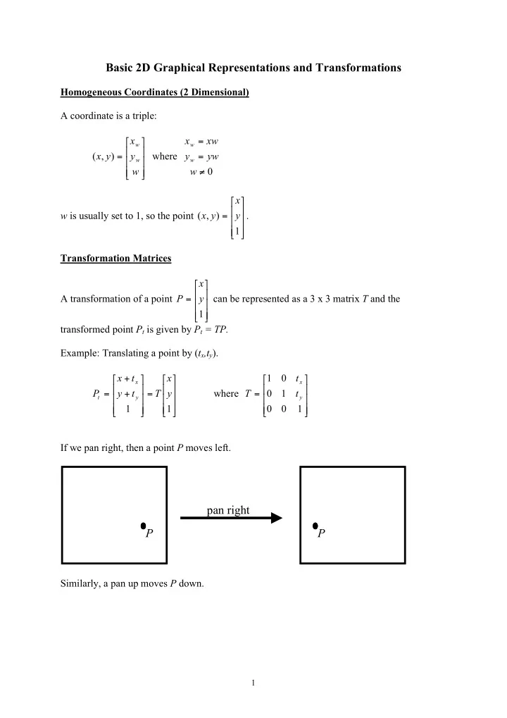
1 y x P can be represented as a 3 x 3 matrix T and the transformed point Pt is given by Pt = TP. Example: Translating a point by (tx,ty).

• =
• +

+ = 1 1 y x T t y t x P

y x t

where

• =

1 1 1

y x

t t T If we pan right, then a point P moves left.

pan right P P

Similarly, a pan up moves P down.

2

So, a pan of p in the x-direction and q in the y-direction gives a transformation matrix:

• =

1 1 1 q p T Zooming Consider a line from

• 1

to

• 1

y x . If we zoom about the point

• 1

so that the line is twice as big, then the line is from

• 1

to

• 1

2 2 y x

• n the display.

If we zoom about the point

• 1

y x , then

• 1

y x doesn’t change on the display. But, the other end of the line moves so that the line is twice as long. So, the line is from

• 1

y x to

• 1

y x

• n the

display. How do we represent this in matrix form? Clearly, the zoom about

• 1

is a simple scale

• =

1 2 2

2

Z and a general scale is

• =

1

y x

s s S Now, a zoom about an arbitrary point P can be made by:

• Translating P to the origin.
• Zooming about the origin.
• Translating the origin back to P.

Note, for

• =

1 y x P

• =

1 1 1 y x Torigin and

• =

1 1 1 y x Tback .

3

But,

• =
• =

1 1 1 1 1 1 1 1 1 y x y x T T

back

• rigin

. So,

back

• rigin

T T =

1

Therefore, a zoom, Z, about P (where Tp translates P to the origin) of a point Q is:

• Translate, TpQ
• Zoom, Z(TpQ)
• Translate back,

Q ZT T Q T Z T

p p p p 1 1

)) ( (

• =

Note, if we are zooming a scene, we can compute

p p ZT

T

1

• first, and then, apply it to all
• points. Also, we don’t need to compute every point. We can compute a clipping rectangle by
• Taking the current window edges as a rectangle, W, in the screen-coordinate system.
• Compute the inverse of the zoom about P,

1 1

• p

p

T Z T .

• Compute a clipping rectangle,

W T Z T W

p p 1 1

'

• =

.

• Objects outside of

' W are not on the display and don’t need to be transformed. In principle, all objects should be kept in a global coordinate system (world coordinates) and each viewport (window) should keep a current transformation matrix V. Now, W V T Z T W

p p 1 1 1

'

• =

4

Cohen-Sutherland Line Clipping

We need an efficient way to clip a picture to the visible window. If one assumes that most

• bjects are represented as collections of lines, then the Cohen-Sutherland line clipping

algorithm is very efficient. Divide the world into a tick-tac-toe (crosses and noughts) board and assign binary bit codes according to the following diagram. Basically, each bit is a 1 if the region lays to the right, above, below, or to the left. Using the diagram, compute the bit codes for the points A and B on the line AB . Now for bit codes a and b from A and B respectively, if a | b = 0 then AB is entirely visible. if a & b ≠ 0 then AB is entirely invisible

• therwise, split the line on a boundary of the visible area and recursively test each new

line segment Visible Region 0000 1100 0100 0010 1000 1010 0101 0001 0011

5

Other Transformations

Other common graphical transformations are also represented in this way. They include: Rotations:

• 1

cos sin sin cos Reflections:

• 1

1 1 about the x-axis

• 1

1 1 about the y-axis

• 1

1 1 relative to the origin (about the z-axis)

• 1

1 1 about the line x=y These can, of course, be combined to reflect about arbitrary lines. For example, the reflection relative to an arbitrary point, ) , ( y x P = , would be obtained by translating it to the origin, reflecting relative to the origin and translating back. Or,

• =
• 1

2 1 2 1 1 1 1 1 1 1 1 1 1 y x y x y x Affine Transforms All of the above are examples of affine transforms. Affine transforms have the property: ) ( ) ( ( TP TQ TP P Q P T

• +

=

• +
• They map the standard affine space of R3 (R3 =

1 : ) , , ( =

• z

z y x ) into itself. The transformation matrices always have inverses. In fact, for a “zoom and pan” transform

6

• 1

y z x z the inverse is

• 1

/ / 1 / / 1 z y z z x z . Which is fortunate because normally computing the inverse of a matrix is computationally expensive. This would mean that computing the clipping window would be expensive as well. Theorem: Combinations of rotations, translations, and scales have inverses. Note, that all are square matrices and have inverses. Let A and B be arbitrary rotations, translations, or scales and AB be an arbitrary combination. Then, A-1 and B-1 exist, and

( )

I AA A BB A A ABB A B AB = = = =

• 1

1 1 1 1 1 1

) )( ( So, B-1A-1 is the inverse of AB and the inverse of the combination exists.

7

Extensions to 3D

Points are represented in the standard homogeneous vector space of R4. That is in the form

• 1

z y x . Similarly, transformations are 4 x 4 matrices. Zoom ⇒

• 1

s s s , Translate ⇒

• 1

1 1 1 z y x One Point Perspective Projection For simplicity, let’s assume that the z-axis goes through the center of the projection plane, is perpendicular to it, and z = 0 in the plane. Then,

• The perspective transformation maps a world point, (x,y,z) along the line between it and

the center of projection. (See the diagram.)

• So, the point (x,y,z) is mapped to (xp,yp) on the projection plan.

8

We can write the projection line in parametric form as: xu x x

• =

' yu y y

• =

' u d z z z ) ( ' +

• =

where 1

• u

if u=0, then (

) ( )

z y x z y x , , ' , ' , ' = . (The point is in the projection plane.) if u=1, then (

) ( )

d z y x , , ' , ' , ' = . (The point is in the same z-plane as the projection point.) Now, on the projection plane '= z . So, we can solve for u. u d z z ) ( +

• =

u d z z ) ( + = ) /( d z z u + = and ) 1 / /( ) /( ) /( ) (( )) /( 1 ( ) /( + = + = +

• +

= +

• =

+

• =

d z x d z xd d z z d z x d z z x d z xz x x p ) 1 / /( ) /( ) /( ) (( )) /( 1 ( ) /( + = + = +

• +

= +

• =

+

• =

d z y d z yd d z z d z y d z z y d z yz y y p =

p

z In matrix form this is:

• +

+ + + ) 1 / /( 1 ) /( 1 ) 1 / /( 1 ) 1 / /( 1 d z d z d z d z Note, perspective projections may be 1, 2, or 3 point. The number of points is controlled by the orientation of the plane

• Plane parallel to 2 principle axes ⇒ 1-point.
• Plane parallel to 1 principle axis ⇒ 2-point.
• Plane parallel to no principle axes ⇒ 3-point.