PageRank (PR) Q: What makes a web page important? A: many important - - PowerPoint PPT Presentation

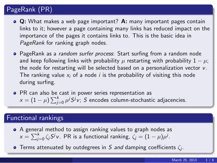
PageRank (PR)

Q: What makes a web page important? A: many important pages contain links to it; however a page containing many links has reduced impact on the importance of the pages it contains links to. This is the basic idea in PageRank for ranking graph nodes. PageRank as a random surfer process: Start surfing from a random node and keep following links with probability µ restarting with probability 1 − µ; the node for restarting will be selected based on a personalization vector v. The ranking value xi of a node i is the probability of visiting this node during surfing. PR can also be cast in power series representation as x = (1 − µ) k

j=0 µjSjv; S encodes column-stochastic adjacencies.

Functional rankings

A general method to assign ranking values to graph nodes as x = k

j=0 ζjSjv. PR is a functional ranking, ζj = (1 − µ)µj.

Terms attenuated by outdegrees in S and damping coefficients ζj.

March 25, 2013 1 / 6

Q: Is there a way to encode functional rankings as surfing processes? A: Multidamping

1-1 1-2 1-κ 1 2 κ

Computing µj in multidamping

Simulate a functional ranking by random surfers following emanating links with probability µj at step j given by : µj = 1 −

1 1+

ρk−j+1 1−µj−1

, j = 1, ..., k, where µ0 = 0 and ρk−j+1 = ζk−j+1

ζk−j

Examples LinearRank (LR) xLR = k

j=0 2(k+1−j) (k+1)(k+2)Sjv : µj = j j+2, j = 1, ..., k.

TotalRank (TR) xTR = ∞

j=0 1 (j+1)(j+2)Sjv : µj = k−j+1 k−j+2, j = 1, ..., k.

Advantages of multidamping

Reduced computational cost in approximating functional rankings using the Monte Carlo approach. A random surfer terminates with probability 1 − µj at step j. Inherently parallel and synchronization free computation.

March 25, 2013 2 / 6

0.5 0.55 0.6 0.65 0.7 0.75 0.8 0.85 0.9 0.95 1 1 2 3 4 5 6 7 8 9 10 Kendall tau step TotalRank: Kendall tau vs step for TopK=1000 nodes (uk-2005) iterations surfers 5 10 15 20 25 30 1e+06 2e+06 3e+06 4e+06 5e+06 6e+06 7e+06 # shared nodes (max=30) microstep Personalized LinearRank: Number of shared nodes (max=30) vs microstep (in-2004). For the seed node 20% of the nodes has better ranking in the Non-Personalized run. iterations surfers

Approximate ranking: Run n surfers to completion for graph size n. How well does the computed ranking capture the “reference” ordering for top-k nodes (Kendall τ, y-axis) in comparison to the one calculated by standard iteration (for a number of steps, x-axis)

• f equivalent computational cost/number of operations? [Left]

Approximate personalized ranking: Run < n surfers to completion (each called a microstep, x-axis), but only from a selected node (personalized). How well can we capture the “reference” top-k nodes, i.e. how many of them are shared (y-axis), compared to the iterative approach of equivalent computational load? [Right]

[uk-2005: 39, 459, 925 nodes, 936, 364, 282 edges. in-2004: 1, 382, 908 nodes, 16, 917, 053 edges]

March 25, 2013 3 / 6

Node similarity: Two nodes are similar if they are linked by other similar node pairs. By pairing similar nodes, the two graphs become aligned. In IsoRank, a state-of-the-art graph alignment method, first a matrix X of similarity scores between the two sets of nodes is computed and then maximum-weight bipartite matching approaches extract the most similar pairs. Let ˜ A, ˜ B the adjacencies AT, BT of the two graphs normalized by columns (network data), Hij independently known similarity scores (preferences matrix) between nodes i ∈ VB and j ∈ VA and µ the percentage of contribution of network data in the algorithm. To compute X, IsoRank iterates: X ← µ ˜ BX ˜ AT + (1 − µ)H

March 25, 2013 4 / 6

Network Similarity Decomposition (NSD)

We reformulate IsoRank iteration and gain speedup and parallelism. In n steps of we reach X (n) = (1 − µ) n−1

k=0 µk ˜

BkH( ˜ AT)k + µn ˜ BnH( ˜ AT)n Assume for a moment that H = uv T (1 component). Two phases for X:

1

u(k) = ˜ Bku and v (k) = ˜ Akv (preprocess/compute iterates)

2

X (n) = (1 − µ) n−1

k=0 µku(k)v (k)T + µnu(n)v (n)T (construct X)

This idea extends to s components, H ∼ s

i=1 wizT i .

NSD computes matrix-vector iterates and builds X as a sum of outer products of vectors; these are much cheaper than triple matrix products. We can then apply Primal Dual Matching (PDM) or Greedy Matching (1/2 approximation, GM) to extract the actual node pairs.

networks matches elemental similarities as component vectors

PDM GM NSD

networks matches elemental similarities as matrix

IsoRank

March 25, 2013 5 / 6

Species Nodes Edges celeg (worm) 2805 4572 dmela (fly) 7518 25830 ecoli (bacterium) 1821 6849 hpylo (bacterium) 706 1414 hsapi (human) 9633 36386 mmusc (mouse) 290 254 scere (yeast) 5499 31898 Species pair NSD (secs) PDM (secs) GM (secs) IsoRank (secs) celeg-dmela 3.15 152.12 7.29 783.48 celeg-hsapi 3.28 163.05 9.54 1209.28 celeg-scere 1.97 127.70 4.16 949.58 dmela-ecoli 1.86 86.80 4.78 807.93 dmela-hsapi 8.61 590.16 28.10 7840.00 dmela-scere 4.79 182.91 12.97 4905.00 ecoli-hsapi 2.41 79.23 4.76 2029.56 ecoli-scere 1.49 69.88 2.60 1264.24 hsapi-scere 6.09 181.17 15.56 6714.00

We computed the similarity matrices X for various possible pairs of species using Protein-Protein Interaction (PPI) networks. µ = 0.80, uniform initial conditions (outer product of suitably normalized 1’s for each pair), 20 iterations, one component. Then we extracted node matches using PDM and GM. 3 orders of magnitude speedup of NSD-based approaches compared to IsoRank

• nes.

Parallelization: NSD has also been ported to parallel/distributed platforms: We have aligned up to million-node graph instances using up to 3, 072 cores in a supercomputer installation. We have managed to process graph pairs of over a billion nodes and twenty billion edges each, over MapReduce-based platforms.

March 25, 2013 6 / 6