P Q 2009 2002 CPI 2009 P Q 2002 2002 CPI includes all - PDF document

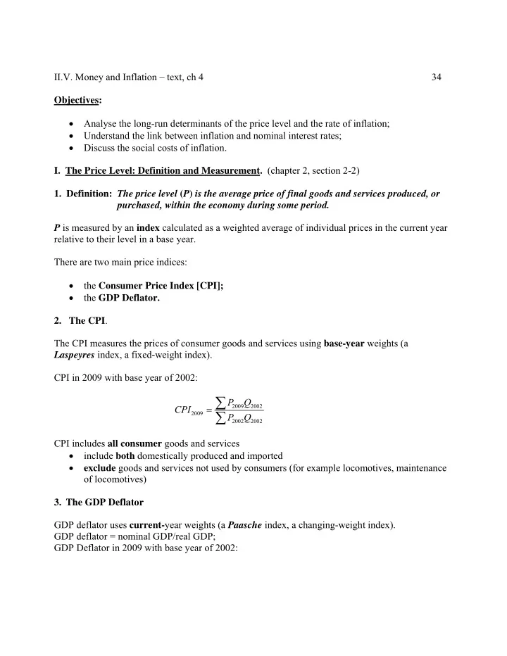
II.V. Money and Inflation – text, ch 4 34 Objectives:  Analyse the long-run determinants of the price level and the rate of inflation;  Understand the link between inflation and nominal interest rates;  Discuss the social costs of inflation. I. The Price Level: Definition and Measurement. (chapter 2, section 2-2) 1. Definition: The price level ( P ) is the average price of final goods and services produced, or purchased, within the economy during some period. P is measured by an index calculated as a weighted average of individual prices in the current year relative to their level in a base year. There are two main price indices:  the Consumer Price Index [CPI];  the GDP Deflator. 2. The CPI . The CPI measures the prices of consumer goods and services using base-year weights (a Laspeyres index, a fixed-weight index). CPI in 2009 with base year of 2002:  P Q  2009 2002 CPI  2009 P Q 2002 2002 CPI includes all consumer goods and services  include both domestically produced and imported  exclude goods and services not used by consumers (for example locomotives, maintenance of locomotives) 3. The GDP Deflator GDP deflator uses current- year weights (a Paasche index, a changing-weight index). GDP deflator = nominal GDP/real GDP; GDP Deflator in 2009 with base year of 2002:

II.V. Money and Inflation – text, ch 4 35  P Q  2009 2009 GDP Deflator  2009 P Q 2002 2009 GDP deflator includes all domestic goods and services. Note: a Laspeyres index (CPI) overstates the rate of inflation. a Paasche index (GDP Deflator) understates it Example: legal services and computers In practice – the rates of inflation calculated with the two indices are fairly close. Differences between CPI and GDP deflator:  CPI uses base-year weights; GDP deflator uses current-year weights;  CPI includes only consumer goods and services; GDP deflator includes all output;  GDP deflator does not include imported goods; CPI includes both domestic and imported goods 4. The rate of inflation = rate of change of a price index . Example: 2008 CPI = 114.1; 2007 CPI = 111.5 (on a base of 100 in 2002) Rate of inflation = (114.1-111.5) x 100 = 2.3% (2007-08) 111.5 Canadian inflation facts: Measured by the percentage change in the CPI, the annual inflation rate has been positive in every year since 1953. The average annual rate of inflation by decade peaked in the 1970s at 7.4%. 1970s 7.4%. 1980's : 6.5% 1990's : 2.2% 2.3% 2000-2011:

II.V. Money and Inflation – text, ch 4 36 II. Money: Nature, Functions, and Control. 1. Definition: Money is a stock of assets directly used in transactions . General definition: The money stock consists of the value of currency [notes + coins] in circulation plus the value of all checking deposits at financial institutions. These – liquid assets, which can be used in transactions Several definitions of money are used: B – monetary base = currency plus chartered bank deposits at the Bank of Canada M1: currency in circulation, demand deposits and other chequing deposits at chartered banks More general definitions: include saving and notice deposits, term deposits etc. What money is NOT :  Money is NOT the same as income : income is a flow of purchasing power, while money is a stock of purchasing power.  Money is NOT the same as wealth : while both money and wealth are stocks, wealth is a broader concept which includes all assets - including money, bonds, equities, real estate, personal property etc. 2. Functions of Money.  Medium of exchange (what we use to buy goods and services; “legal tender”)  Unit of account (how prices are quoted and debts recorded; no alternative)  Store of value (one of a number of ways a way of transferring purchasing power from present to the future) 3. Types of Money .  Fiat (no intrinsic value, e.g. paper money)  commodity (intrinsic value, e.g. Gold standard - when gold was the commodity.) How fiat money evolves:  initially people use pure gold, but verification is difficult;  to reduce verification costs specialists convert gold into gold coins - their fee is called

II.V. Money and Inflation – text, ch 4 37 seigniorage ;  to reduce the weight carried around the govt. takes your gold and issues gold certificates - banknotes. It promises to convert certificates for gold without limit;  government issues more certificates than gold it gets; still promises to exchange certificates for gold; seigniorage increases;  government stops exchanging banknotes for gold but makes the money legal tender; seigniorage increases further. 4. Control of the Quantity of Money.  Is the responsibility of Canada’s central bank - the Bank of Canada.  Decisions - are the responsibility of the Governor of the Bank of Canada with input from the Federal Minister of Finance and constitute the govt’s monetary policy .  The main method of control of the money supply is through open market operations - purchase or sale of outstanding govt. bonds by the Bank of Canada;  the Bank of Canada - increases the money supply by buying bonds from the public - decreases the money supply by selling bonds to the public. III. The Quantity Theory of Money (QTM). 1. Transactions and the Quantity Equation The size of money stock [ M ] required to transact the purchase and sale of a given flow of output depends on three factors:  The volume of output per period [ Y ]  The price of a typical unit of output or the GDP Deflator [ P ]  The [income] velocity of circulation of money : the number of times each period a unit of M is used to purchase output, or is received as income, each period [ V ]. The Quantity Equation: M V = P Y Note: The quantity equation is an identity - a relationship which is “true by definition” - because we defined velocity [ V ] to meet this equation. Example: Assume there is single final good: beer; 100 bottles sold daily; price $1.25 each; $50 of money

II.V. Money and Inflation – text, ch 4 38 in circulation: P =$1.25, Y =100, M =50 So: V = $125/$50 = 2.5 2. QTM as a theory of Nominal GDP. We can use the Quantity Theory of Money as a theory of nominal GDP. We assume: V  V (i) income velocity constant : M  M (ii) the nominal money supply is exogenous: So:  M V PY Conclusion: Given constant velocity, the quantity of money ( M ) determines nominal GDP ( PY ): a change in the quantity of money ( M ) causes a proportionate change in nominal GDP ( PY ). 3. QTM as a theory of the price level and inflation. The idea is as follows. In the long run, the level of output does not depend on the quantity of money in the economy. We will discuss this in more detail later. So Y  Y Assume constant velocity. Then M determines nominal output ( PY ). P is the ratio of nominal to the constant real output: M V P  Y Conclusion: For given values of velocity and real GDP, the price level ( P ) varies directly with the money stock ( M ): a change in M causes a proportionate change in P . The equation is in absolute terms. It says that if real GDP and velocity are constant, the price level changes one for one with the money supply.

II.V. Money and Inflation – text, ch 4 39 In actual economies real GDP changes over time; velocity may also change. So it is useful to express the quantity theory equation in terms of percentage change. To do this, we use a very simple and easy to remember formula: The percentage change of a product of two variables = the sum of percentage changes of these variables So: the percentage change of MV = the percentage change of M plus the percentage change of V Using this formula:        % M % V % P % Y  % P Rearranging terms we obtain the expression for the inflation rate, :        % P % M % V % Y  V  % 0 Assuming, constant velocity:      % P % M % Y � is the rate of growth of the money suppy and %∆� � is the rate of growth of output. Here %∆� Conclusion: For a given rate of economic growth, and assuming constant velocity, the higher is the rate of growth of the money supply, the higher is the rate of inflation. Evidence: across countries - Fig. 4-2 US - decades - Fig. 4-1 IV. Inflation and Nominal Interest Rates. 1. Real vs nominal interest rates. i = nominal interest rate, or the cost of borrowing/ reward to lending, measured in dollars; r = real interest rate, or the cost of borrowing/reward to lending, measured in goods.