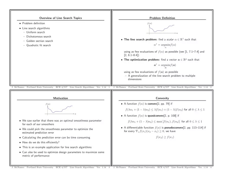
overview of line search topics problem definition problem
play

Overview of Line Search Topics Problem Definition Problem - PowerPoint PPT Presentation

Overview of Line Search Topics Problem Definition Problem definition f ( ) Line search algorithms Uniform search Dichotomous search The line search problem: find a scalar R 1 such that Golden section search


  1. Overview of Line Search Topics Problem Definition • Problem definition f ( α ) • Line search algorithms – Uniform search α – Dichotomous search • The line search problem: find a scalar α ∈ R 1 such that – Golden section search α ∗ = argmin f ( α ) – Quadratic fit search α using as few evaluations of f ( α ) as possible (see [1, 7.1–7.4] and [2, 8.1–8.4]) • The optimization problem: find a vector a ∈ R p such that a ∗ = argmin f ( a ) α using as few evaluations of f ( a ) as possible – A generalization of the line search problem to multiple dimensions J. McNames Portland State University ECE 4/557 Line Search Algorithms Ver. 1.14 1 J. McNames Portland State University ECE 4/557 Line Search Algorithms Ver. 1.14 2 Motivation Convexity • A function f ( α ) is convex [2, pp. 79] if f ( α ) f ( λα 1 + (1 − λ ) α 2 ) ≤ λf ( α 1 ) + (1 − λ ) f ( α 2 ) for all 0 ≤ λ ≤ 1 α • A function f ( α ) is quasiconvex [2, p. 108] if • We saw earlier that there was an optimal smoothness parameter f ( λα 1 + (1 − λ ) α 2 ) ≤ max [ f ( α 1 ) , f ( α 2 )] for all 0 ≤ λ ≤ 1 for each of our smoothers • A differentiable function f ( α ) is pseudoconvex [2, pp. 113–114] if • We could pick the smoothness parameter to optimize the for every ∇ x f ( x 1 )( x 2 − x 1 ) ≥ 0 , we have estimated prediction error f ( x 2 ) ≥ f ( x 1 ) • Calculating the prediction error can be time consuming • How do we do this efficiently? • This is an example application for line search algorithms • Can also be used to optimize design parameters to maximize some metric of performance J. McNames Portland State University ECE 4/557 Line Search Algorithms Ver. 1.14 3 J. McNames Portland State University ECE 4/557 Line Search Algorithms Ver. 1.14 4

  2. Goal Interval Bounding Problem f ( α ) f ( α ) α α • There is no line search algorithm that is guaranteed to find the • Many line search algorithms try to find a local minimum in the range [0 , ∞ ] as quickly as possible global minimum for any function f ( α ) • If the criteria contains multiple local minima, they find one of • All of the line search algorithms try to find a possibly local them quickly minimum as quickly as possible • Otherwise they find the global minima • They are designed with functions with some type of convexity in mind • Most of these algorithms require that the minima be constrained to a finite range: α ∗ ∈ [ α min , α max ] • Work with non-convex functions, but very few compare or try to find the deepest local minimum • By the nature of the problem, the lower limit is usually known to be zero: α min = 0 • Many heuristic techniques for searching for the global minimum, but none provide any guarantees or any claims of optimality • Often the upper limit has to be found J. McNames Portland State University ECE 4/557 Line Search Algorithms Ver. 1.14 5 J. McNames Portland State University ECE 4/557 Line Search Algorithms Ver. 1.14 6 Interval Bounding Algorithm Example 1: Interval Bounding This is one popular algorithm for finding the upper limit for a line 1 search algorithm. The user specifies the initial step α 1 and picks the expansion rate c . 0.8 • Evaluate the function at α 0 = 0 • Evaluate the function at α 1 0 0.6 • Evaluate the function at α 2 = α 1 × c f ( α ) • k = 1 4 0.4 • Until f ( α k − 1 ) > f ( α k ) and f ( α k ) < f ( α k +1 ) 1 – k := k + 1 2 3 0.2 – α k +1 := α k × c • There is a minimum between α k − 1 and α k +1 0 0 0.1 0.2 0.3 0.4 0.5 0.6 0.7 0.8 0.9 1 Note that this algorithm may also increase the lower bound from its α initial value of 0. J. McNames Portland State University ECE 4/557 Line Search Algorithms Ver. 1.14 7 J. McNames Portland State University ECE 4/557 Line Search Algorithms Ver. 1.14 8

  3. Example 1: MATLAB Code for c1 = 1: length(x), h = text(x(c1 )+0.01 ,LSFn(x(c1)), num2str(c1 -1)); set(h,’HorizontalAlignment ’,’Left ’); set(h,’VerticalAlignment ’,’Middle ’); end function [] = IntervalBound ; box off; FigureLatex; st = 2; % Step size xlabel(’ α ’); x = zeros (100 ,1); ylabel(’ f ( α ) ’); x(1) = 0; AxisSet (8); x(2) = 0.1; % First step x(3) = x(2)* st; print -depsc IntervalBound ; cnt = 3; while ¬ (LSFn(x(cnt -2)) > LSFn(x(cnt -1)) & LSFn(x(cnt -1)) < LSFn(x(cnt ))) cnt = cnt + 1; x(cnt) = x(cnt -1)* st; end x = x(1: cnt ); x0 = x(cnt -2); x1 = x(cnt ); figure; FigureSet (1,’Slides ’); u = 0:0 .01 :1; h = patch ([x0 x1 x1 x0],[0 0 1 1],’k’); set(h,’LineStyle ’,’None ’); set(h,’FaceColor ’,0.8 *[1 1 1]); % Light gray region hold on; h = plot(u,LSFn(u),’r’,x,LSFn(x),’.’); set(h(2),’MarkerSize ’ ,8); set(h,’LineWidth ’,1.2); hold off; J. McNames Portland State University ECE 4/557 Line Search Algorithms Ver. 1.14 9 J. McNames Portland State University ECE 4/557 Line Search Algorithms Ver. 1.14 10 Bounding the Line Search Interval Uniform Search More generally, the line search interval can be found by “interval f ( α ) doubling”. Assume that α is constrained to being a positive number. 1. Pick initial values of α min α 2. While f ( α min ) < f ( α max ) , α min = α min /c • Pick the search points α 1 , α 2 , . . . , α n so that they are uniformly 3. While f ( α min ) > f ( α max ) , α max = α max × c spaced over some preset range Typically c = 2 , but any c > 1 could be used. • Then pick the best α α ∗ = argmin α ∈{ a 1 ,a 2 ,...,a n } f ( α ) + No assumptions about convexity or shape of f ( α ) + Finds (nearly) a global minimum − Relatively inefficient J. McNames Portland State University ECE 4/557 Line Search Algorithms Ver. 1.14 11 J. McNames Portland State University ECE 4/557 Line Search Algorithms Ver. 1.14 12

  4. Example 2: Uniform Search Example 2: MATLAB Code Resolution:0.2222 1 function [] = UniformSearch ; ll = 0; % Lower limit ul = 1; % Upper limit np = 10; % No. of points 0.8 x = ll:(ul -ll)/(np -1): ul; f = LSFn(x); xrng = (ul -ll )/(np -1); 0.6 [fmin ,id] = min(f); f ( α ) xmin = x(id); figure; 0.4 FigureSet (1,’Slides ’); u = 0:0 .01 :1; h = plot(u,LSFn(u),’r’,x,f,’.’,xmin ,fmin ,’g.’); set(h(2),’MarkerSize ’ ,8); set(h,’LineWidth ’,1.2); 0.2 set(h(3),’MarkerSize ’ ,15); box off; st = sprintf(’Resolution :%6 .4f ’ ,2*min(diff(x))); title(st); FigureLatex; 0 xlabel(’ α ’); 0 0.1 0.2 0.3 0.4 0.5 0.6 0.7 0.8 0.9 1 ylabel(’ f ( α ) ’); α AxisSet (8); print -depsc UniformSearch ; J. McNames Portland State University ECE 4/557 Line Search Algorithms Ver. 1.14 13 J. McNames Portland State University ECE 4/557 Line Search Algorithms Ver. 1.14 14 Dichotomous Search Example 3: Dichotomous Search • Suppose you know that α is in the range of α min to α max Resolution:0.0332 1. Calculate the following evaluation points 1 b = α min + α max c = α min + α max − ǫ + ǫ 2 2 0.8 2. If f ( b ) < f ( c ) , set α max = c Otherwise, set α min = b 0.6 3. Repeat until convergence f ( α ) • If the derivative d f ( α ) can be calculated, the computation can be 0.4 d α reduced to one evaluation of the derivative per an iteration 5 3 7 9 • If the derivative is used, this is called the bisection method 0.2 − Converges to a local minimum (global if f ( α ) is quasiconvex) 1 + Faster than a uniform search 0 0 0.1 0.2 0.3 0.4 0.5 0.6 0.7 0.8 0.9 1 α J. McNames Portland State University ECE 4/557 Line Search Algorithms Ver. 1.14 15 J. McNames Portland State University ECE 4/557 Line Search Algorithms Ver. 1.14 16

  5. Example 3: Dichotomous Error Example 3: MATLAB Code 0.25 function [] = DichotomousSearch ; clear all; close all; 0.2 ll = 0; % Lower limit ul = 1; % Upper limit np = 10; % No. of points eta = 0.001; % Dither 0.15 f ( α i ) cnt = 0; x = zeros(np ,1); f = zeros(np ,1); 0.1 for c1 = 1:np/2, mp = (ul+ll )/2; b = mp -eta; fb = LSFn(b); c = mp+eta; fc = LSFn(c); if fb <fc , 0.05 ul = c; else ll = b; end; 0 cnt = cnt + 1; 1 2 3 4 5 6 7 8 9 10 x(cnt) = b; f(cnt) = fb; Iteration cnt = cnt + 1; x(cnt) = c; f(cnt) = fc; end; J. McNames Portland State University ECE 4/557 Line Search Algorithms Ver. 1.14 17 J. McNames Portland State University ECE 4/557 Line Search Algorithms Ver. 1.14 18 [fmin ,id] = min(f); xlim ([0 .5 length(f)+0 .5 ]); xmin = x(id); ylim ([0 1.05*max(f)]); xrng = ul -ll; FigureLatex; ylabel(’ f ( αk ) ’); figure; xlabel(’Iteration (k)’); FigureSet (1,’Slides ’); box off; u = 0:0 .01 :1; AxisSet (8); h = plot(u,LSFn(u),’r’,x,f,’.’,xmin ,fmin ,’g.’); print -depsc DichotomousError; set(h(2),’MarkerSize ’ ,8); set(h,’LineWidth ’,1.2); set(h(3),’MarkerSize ’ ,15); for c1 = 1:2: length(x), h = text(x(c1),f(c1 )+0.01 ,num2str(c1 )); set(h,’HorizontalAlignment ’,’Center ’); set(h,’VerticalAlignment ’,’Bottom ’); end; FigureLatex; xlabel(’ α ’); ylabel(’ f ( α ) ’); st = sprintf(’Resolution :%6 .4f\n’,xrng ); title(st); box off; AxisSet (8); print -depsc DichotomousSearch ; figure; FigureSet (2,’Slides ’); k = 1: length(f); u = 0:0 .01 :1; h = stem(k,f,’r’); set(h,’MarkerFaceColor ’,’r’); J. McNames Portland State University ECE 4/557 Line Search Algorithms Ver. 1.14 19 J. McNames Portland State University ECE 4/557 Line Search Algorithms Ver. 1.14 20

Download Presentation
Download Policy: The content available on the website is offered to you 'AS IS' for your personal information and use only. It cannot be commercialized, licensed, or distributed on other websites without prior consent from the author. To download a presentation, simply click this link. If you encounter any difficulties during the download process, it's possible that the publisher has removed the file from their server.

Recommend


More recommend