Overview Neural networks and visual processing So far we have - - PowerPoint PPT Presentation

Neural networks and visual processing

Mark van Rossum

School of Informatics, University of Edinburgh

January 24, 2018

0Version: January 24, 2018. 1 / 71

Overview

So far we have discussed unsupervised learning up to V1 For most technology applications (except perhaps compression), V1 description is not enough. Yet it is not clear how to proceed to higher areas. At some point supervised learning will be necessary to attach

• labels. Hopefully this can be postponed to very high levels.

2 / 71

Neurobiology of Vision

WHAT pathway: V1 → V2 → V4 → IT (focus of our treatment) WHERE pathway: V1 → V2 → V3 → MT/V5 → parietal lobe IT (Inferotemporal cortex) has cells that are

Highly selective to particular objects (e.g. face cells) Relatively invariant to size and position of objects, but typically variable wrt 3D view

What and where information must be combined somewhere (’throw the ball at the dog’)

3 / 71

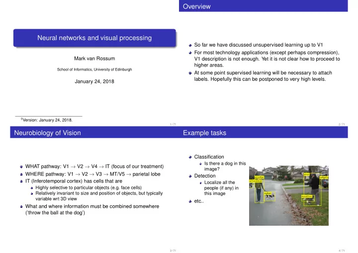
Example tasks

Classification

Is there a dog in this image?

Detection

Localize all the people (if any) in this image

etc..

4 / 71

Invariances in higher visual cortex

[Logothetis and Sheinberg, 1996]

5 / 71

Invariance is however limited

Left: partial rotation invariance [Logothetis and Sheinberg, 1996]. Right: clutter reduces translation invariance [Rolls and Deco, 2002].

6 / 71

Computational Object Recognition

The big problem is creating invariance to scaling, translation, rotation (both in-plane and out-of-plane), and partial occlusion, yet at the same time being selective. Large input dimension, need enormous (labelled) training set + tricks Objects are not generally presented against a neutral background, but are embedded in clutter Within class variation of objects (e.g. cars, handwritten letters, ..)

7 / 71

Geometrical picture

[From Bengio 2009 review] Pixel space. Same objects form manifold (potentially discontinuous, and disconnected).

8 / 71

Some Computational Models

Two extremes: Extract 3D description of the world, and match it to stored 3D structural models (e.g. human as generalized cylinders) Large collection of 2D views (templates) Some other methods 2D structural description (parts and spatial relationships) Match image features to model features, or do pose-space clustering (Hough transforms))

What are good types of features?

Feedforward neural network Bag-of-features (no spatial structure; but what about the “binding problem”?) Scanning window methods to deal with translation/scale

9 / 71

AI

[Bengio et al., 2014]

10 / 71

History

McCullough & Pitts (1943): Binary neurons can implement any finite state machine. Von Neumann used this for his architecture. Rosenblatt (1962): Perceptron learning rule: Learning of (some) binary classification problems. Backprop (1980s): Universal function approximator. Generalizes, but has local maxima. Boltzmann machines (1980s): Probabilistic models. Long ignored for being exceedingly slow.

11 / 71

Perceptrons

Supervised binary classification of K N-dimensional xµ pattern vectors. y = H(h) = H(w.x + b), H is step function, h = w.x + b is net input (’field’) [ignore Ai in figure for now, and assume xi is pixel intensity]

12 / 71

Perceptron learning rule

Denote desired binary output for pattern µ as dµ. Rule: ∆wµ

i = ηxµ i (dµ − yµ)

• r, to be more robust, with margin κ

∆wµ

i = ηH(Nκ − hµdµ)dµxµ i

note, if patterns correct then ∆wµ

i = 0 (stop-learning).

If learnable, rule converges in polynomial time.

13 / 71

Perceptron learning rule

Learnable if patterns are linearly separable. Random patterns are typically learnable if #patterns < 2.#inputs, K < 2N. Mathematically solves set of inequalities. General trick: replace bias b = wb.1 with ’always on’ input.

14 / 71

Perceptron biology

Tricky questions How is the supervisory signal coming into the neuron? How is the stop-learning implemented in Hebbian model where ∆wi ∝ xiy? Perhaps related to cerebellar learning (Marr-Albus theory)

15 / 71

Perceptron and cerebellum

16 / 71

Perceptron and cerebellum

17 / 71

[Purkinje cell spikes recorded extra-cellularly + zoom] Simple spikes: standard output. Complex spikes: IO feedback, trigger plasticity.

18 / 71

Perceptron limitation

1

Perceptron with limited receptive field cannot determine connectedness (give output 1 for connected patterns and 0 for dis-connected). This is the XOR problem, d = 1 if x1 = x2. This is the simplest parity problem, d = (

i xi)mod2.

Equivalently, identity function problem, d = 1 if x1 = x2. In general: categorizations that are not linearly separable cannot be learned (weight vector keeps wandering).

19 / 71

Multi-layer perceptron (MLP)

Supervised algorithm that overcomes limited functions of the single perceptron. With continuous units and large enough single hidden layer, MLP can approximate any continuous function! (and two hidden layers approximate any function). Argument: write function as sum of localized bumps, implement bumps in hidden layer. Ultimate goal is not the learning of the patterns (after all we could just make a database), but a sensible generalization. The performance on test-set, not training set, matters.

20 / 71

yµ

i (xµ; w, W) = g( j Wijvj) = g

• j Wijg(

k wjkxk)

• Learning: back-propagation of errors. Mean squared error of P

training patterns: E =

P

• µ=1

Eµ = 1 2

P

• µ=1

[dµ

i − yµ i (xµ; w, W)]2

Gradient descent (batch) ”∆w ∝ −η ∂E

∂w ” where w are all the

weights (input → hidden, hidden → output, biases).

21 / 71

Stochastic descent: Pick arbitrary pattern, use ∆w = −η ∂Eµ

∂w

instead of ∆w = −η ∂E

∂w . Quicker to calculate, and randomness

helps learning.

∂Eµ ∂Wij = (yi − di)g′( k Wikvk)vj ≡ δivj ∂Eµ ∂wjk = i δiWijg′( l wjlxl)xk

Start from random, smallish weights. Convergence time depends strongly on lucky choice. If g(x) = [1 + exp(−x)]−1, one can use g′(x) = g(x)(1 − g(x)). Normalize input (e.g. z-score)

22 / 71

MLP tricks

Learning MLPs is slow and local maxima are present. [from HKP , increasing learning rate. 2nd: fastest, 4th: too big] Learning rate often made adaptive (first large, later small). Sparseness priors are often added to prevent large negative weights cancelling large positive weights. e.g E = 1

2

• µ(dµ − yµ(xµ; w))2 + λ

i,j w2 ij

Other cost functions are possible. Traditionally one hidden layer. More layers do not enhance repertoire and slow down learning (but see below).

23 / 71

MLP tricks

Momentum: previous update is added, hence wild direction fluctuations in updates are smoothed. [from HKP . Same learning rate but with (right) and without momentum (left)].

24 / 71

MLP examples

Essentially curve fitting. Best on problems that are not fully understood / hard to formulate. Hand-written postcodes. Self-driving car at 5km/h (∼ 1990) Backgammon game

25 / 71

MLP sequence data

Temporal patterns by for instance setting input vector as {s1(t), s2(t), . . . sn(t), s1(t − 1), . . . sn(t − 1)}. Context units that decay over time (Ellman net)

26 / 71

Auto-encoders

Autoencoders: Minimize E(input, output) Fewer hidden units than input units: find optimal compression (PCA when using linear units).

27 / 71

Biology of back-propagation?

How to back-propagate in biology? O‘Reilly (1996) Adds feedback weights (do not have to be exactly symmetric). Uses 2-phases. -phase: input clamped; +phase: input and output clamped. Approximate ∆wij = η(post+

i − post− i )pre− j

more when doing Boltzmann machines...

28 / 71

Convolutional networks

Neocognitron [Fukushima, 1980, Fukushima, 1988, LeCun et al., 1990] To implement location invariance, “clone” (or replicate) a detector

• ver a region of space (weight-sharing), and then pool the

responses of the cloned units This strategy can then be repeated at higher levels, giving rise to greater invariance and faster training

29 / 71

HMAX model

[Riesenhuber and Poggio, 1999] 30 / 71

HMAX model

Deep, hard-wired network S1 detectors based on Gabor filters at various scales, rotations and positions S-cells (simple cells) convolve with local filters C-cells (complex cells) pool S-responses with maximum No learning between layers ! Object recognition: Supervised learning on the output of C2 cells.

31 / 71

Rather than learning, take refuge in having many, many cells. (Cover, 1965)A complex pattern-classification problem, cast in a high-dimensional space non-linearly, is more likely to be linearly separable than in a low-dimensional space, provided that the space is not densely populated.

32 / 71

[Riesenhuber and Poggio, 1999] 33 / 71

HMAX model: Results

“paper clip” stimuli Broad tuning curves wrt size, translation Scrambled input image does not give rise to object detections: not all conjunctions are preserved

34 / 71

More recent version

[Serre et al., 2007]

35 / 71

Use real images as inputs S-cells convolution,e.g. h = (

• i wixi

κ+√

i w2 i

), y = g(h). C-cell soft-max pooling h =

xq+1

i

κ+

k xq i

(some support from biology for such pooling) Some unsupervised learning between layers [Serre et al., 2005]

36 / 71

HMAX model: Results

Localization can be achieved by using a sliding-window method Claimed as a model on a “rapid categorization task”, where back-projections are inactive Performance similar to human performance on flashed (20ms) images The model doesn’t do segmentation (as opposed to bounding boxes)

37 / 71

Learning invariances

Hard-code (convolutional network) http://yann.lecun.com/exdb/lenet/ Supervised learning (show samples and require same output) Use temporal continuity of the world. Learn invariance by seeing

• bject change, e.g. it rotates, it changes colour, it changes shape.

Algorithms: trace rule[Földiák, 1991] E.g. replace ∆w = x(t).y(t) with ∆w = x(t).˜ y(t) where ˜ y(t) is temporally filtered y(t). Similar principles: VisNet [Rolls and Deco, 2002], Slow feature analysis.

38 / 71

Slow feature analysis

Find slow varying features, these are likely relevant [Wiskott and Sejnowski, 2002] Find output y for which: ( dy(t)

dt )2 minimal,

while y = 0, y2 = 1

39 / 71

Experiments: Altered visual world [Li and DiCarlo, 2010]

40 / 71

Including top-down interaction

Extensive top-down connections everywhere in the brain One known role: attention. For the rest: many theories [Epshtein et al., 2008] Local parts can be ambiguous, but knowing global object at helps. Top-down to set priors. Improvement in object recognition is actually small, but recognition and localization of parts is much better.

41 / 71

Deep MLPs

Traditional MLPs are also called shallow (1 or 2 hidden layers). While deeper nets do not have more computational power. 1) Some tasks require less nodes (e.g. 1 hidden layer: parity requires exp. many hidden layer units) 2) they can lead to better

• representations. Better representations lead to better

generalization and better learning. Learning slows down in deep networks, as transfer functions g() saturate at 0 or 1. (∆w ∝ g′() → 0) So:

Pre-training, e.g. with Boltzmann machines (see below) Convolutional networks Use non-saturating activation function.

Better representation by adding noisy/partial stimuli. This artificially increases the training set and forces invariances.

42 / 71

AI

[Bengio et al., 2014]

43 / 71

Role of representation

Finding good representation solves most problems 90% Similarly, bad representation can make problem very hard. E.g. odd/even number categorization using base-2 (only last bit matters ) vs base-3 (all bits matter) representation. E.g. recognition of images after fixed, random scrambling is difficult for humans. This is the task naive MLPs are faced with.

44 / 71

Recurrent networks

MLPs have no dynamics Recurrent networks are dynamic. Could be steady state(s), periodic, or chaotic. With symmetric weights there can only be fixed points (point or line attractors). In recurrent networks it is much harder to find weights to be

• altered. Often restrict to cases where dynamics has fixed points.

45 / 71

Recurrent networks: Hopfield networks

All to all connected network (can be relaxed) Binary units si = ±1, or rate with sigmoidal transfer. Dynamics si(t + 1) = sign[

j wijsj(t)] or continuous version dr(t) dt

= −r + g(Wr(t)). Using symmetric weights wij = wji, we can define energy E = − 1

2

• ij siwijsj.

46 / 71

Under these conditions network moves from initial condition (stimulus, s(t = 0) = x) into the closest attractor state (’memory’) and stays there. Auto-associative, pattern completion Simple (suboptimal) learning rule: wij = M

µ xµ i xµ j

(µ indexes patterns xµ).

47 / 71

Indirect experimental evidence using maze deformation[Wills et al., 2005]

48 / 71

Winner-less competition

How to escape from attractor states? Noise, asymmetric connections, adaptation. From [Ashwin and Timme, 2005].

49 / 71

Liquid state machines

[Maass et al., 2002] Motivation: arbitrary spatio-temporal computation without precise design. Create pool of spiking neurons with random connections. Results in very complex dynamics if weights are strong enough Similar to echo state networks (but those are rate based). Both are known as reservoir computing Similar theme as HMAX model: create rich repetoire and only learn at the output layer.

50 / 71

Various functions can be implemented by varying readout.

51 / 71

Optimal reservoir?

Best reservoir has rich yet predictable dynamics. Edge of Chaos [Bertschinger and Natschlaeger, 2004] Network 250 binary nodes, wij = N(0, σ2) (x-axis is recurrent strength)

52 / 71

Optimal reservoir?

Task: Parity(in(t), in(t − 1), in(t − 2)) Best (darkest in plot) at edge of chaos. Does chaos exist in the brain? In spiking network models: yes [van Vreeswijk and Sompolinsky, 1996] In real brains: ?

53 / 71

Relation to Support Vector Machines

Map problem in to high dimensional space F; there it often becomes linearly separable. This can be done without much computational overhead (kernel trick).

54 / 71

Boltzmann machines

Hopfield network is not perfect. It is impossible to learn only (1, 1, −1), (−1, −1, −1), (1, −1, 1), (−1, 1, 1) but not (−1, −1, 1), (1, 1, 1), (−1, 1, −1), (1, −1, 1) (XOR again)... Because xi =

• xixj
• = 0

Boltmann machines have ±1 units and include two, somewhat unrelated, modifications: Introduce hidden units, these can extract abstract features.

55 / 71

Boltzmann machines

Stochastic updating: p(si = 1) =

1 1+e−2βEi

Ei =

j wijsj − θi, E = i Ei.

T = 1/β is temperature (set to some arbitrary value). Boltzmann distribution P(s) = exp(−βE(s)) Z where Z =

s exp(−βE(s))

56 / 71

Boltzmann machines

Boltzmann machine learns arbitrary P(v). Can thus be used for auto-association (pattern completion) Or, by labelling some visible units as inputs and others as output, can be used as if it were a associator like an MLP .

57 / 71

Learning in Boltzmann machines

The generated probability for state sα, after equilibrium is reached, is given by the Boltzmann distribution Pα = 1 Z

• γ

e−βHαγ Hαγ = −1 2

• ij

wijsisj Z =

• αβ

e−βHαγ where α labels states of visible units, γ the hidden states.

58 / 71

As in other generative models, we match true distribution to generated

• ne. Minimize KL divergence between input and generated

distribution. KL =

• α

Gα log Gα Pα Minimize to get [Ackley et al., 1985, Hertz et al., 1991] ∆wij = ηβ[

• sisj
• clamped −
• sisj
• free]

(note, wij = wji) Wake (’clamped’) phase vs. sleep (’dreaming’) phase Clamped phase: Hebbian type learning. Average over input patterns and hidden states. Sleep phase: unlearn erroneous correlations. The hidden units will ’discover’ statistical regularities.// Biology of phases unknown.

59 / 71

Boltzmann machines: applications

Shifter circuit. Learning symmetry [Sejnowski et al., 1986]. Create a network that categorizes horizontal, vertical, diagonal symmetry (2nd order predicate).

60 / 71

Boltzmann machines: auto-encoders

Autoencoders: Minimize E(input, output) Fewer hidden units than input units: find optimal compression (PCA). More hidden units: impose for instance sparseness.

61 / 71

Restricted Boltzmann

Need for multiple relaxation runs for every weight update (triple loop), makes training Boltzmann networks very slow. Speed up learning in restricted Boltzmann: No hidden-hidden connections Don’t wait for the sleep state to fully settle, one step is enough. Stack multiple layers (deep-learning) Application: high quality auto-encoder (i.e. compression) [Hinton and Salakhutdinov, 2006] [also good webtalks/tutorials by Hinton on this]

62 / 71

Sparse deep belief net model for visual area V2

[Lee et al., 2008] Consider an RBM with Gaussian visible units E(u, v) = 1 2σ2

• i

u2

i − 1

σ2  

i

ciui +

• j

bjvj +

• i,j

uivjwij   p(ui|v) ∼ N(ci +

j wijvj, σ2)

Also impose a sparsity prior on the hidden units, with target sparseness p

• j

||p − 1 m

m

• k=1

E[v(k)

j

|u(k)]||2 Layer 2 trained after layer 1 has learned (DBN)

63 / 71

First layer filters Second layer: each unit “looks at” a small number of first layer units, e.g.

The leftmost patch in each group is a visualization of the model V2 basis, obtained by taking a weighted linear combination of the first layer bases to which it is connected.

Properties of “V2” units can be compared to neural data.

64 / 71

Recurrent models: Ising model of neural activity

To describe data of retinal network, use Ising model [Schneidman et al., 2006] P(r) = 1 Z e(−

i hiri− ij wijrirj)

(But maybe it does not work well in large networks [Roudi et al., 2009])

65 / 71

Generative models

[Berkes et al., 2011] During development spontaneous activity matched stimulus-evoked activity better and better.

66 / 71

References I

Ackley, D., Hinton, G., and Sejnowski, T. (1985). A learning algorithm for Boltzmann machines,. Cognitive Science, 9:147–169. Ashwin, P . and Timme, M. (2005). Nonlinear dynamics: when instability makes sense. Nature, 436(7047):36–37. Bengio, Y., Goodfellow, I. J., and Courville, A. (2014). Deep learning. Book in preparation for MIT Press. Berkes, P ., Orban, G., Lengyel, M., and Fiser, J. (2011). Spontaneous cortical activity reveals hallmarks of an optimal internal model of the environment. Science, 331(6013):83–87. Bertschinger, N. and Natschlaeger, T. (2004). Real-time computation at the edge of chaos in recurrent neural networks. Neural Comput, 16(7):1413–1436. Epshtein, B., Lifshitz, I., and Ullman, S. (2008). Image interpretation by a single bottom-up top-down cycle. Proc Natl Acad Sci U S A, 105(38):14298–14303.

67 / 71

References II

Földiák, P . (1991). Learning invariance from transformation sequences. Neural Comp., 3:194–200. Fukushima, K. (1980). Neocognitron: A self-organising multi-layered neural network. Biol Cybern, 20:121–136. Fukushima, K. (1988). Neocognitron: A hierarchical neural network capable of visual pattern recognition. Neural Networks, 1:119–130. Hertz, J., Krogh, A., and Palmer, R. G. (1991). Introduction to the theory of neural computation. Perseus, Reading, MA. Hinton, G. E. and Salakhutdinov, R. R. (2006). Reducing the dimensionality of data with neural networks. Science, 313(5786):504–507. LeCun, Y., Boser, B., Denker, J. S., Henderson, D., Howard, R. E., Hubbard, W., and Jackel,

• L. D. (1990).

Handwritten digit recognition with a back-propagation network. In Advances in Neural Information Processing Systems 2. Morgan Kaufmann.

68 / 71

References III

Lee, H., Ekanadham, C., and Ng, A. (2008). Sparse deep belief net model for visual area v2. NIPS, 20. Li, N. and DiCarlo, J. J. (2010). Unsupervised natural visual experience rapidly reshapes size-invariant object representation in inferior temporal cortex. Neuron, 67(6):1062–1075. Logothetis, N. K. and Sheinberg, D. L. (1996). Visual object recognition. Annu Rev Neurosci, 19:577–621. Maass, W., Natschlaeger, T., and Markram, H. (2002). Real-time computing without stable states: a new framework for neural computation based

• n perturbations.

Neural Comput, 14(11):2531–2560. Riesenhuber, M. and Poggio, T. (1999). Hierarchical models of object recognition in cortex.

• Nat. Neuro., 2:1019–1025.

Rolls, E. T. and Deco, G. (2002). Computational neuroscience of vision. Oxford.

69 / 71

References IV

Roudi, Y., Aurell, E., and Hertz, J. A. (2009). Statistical physics of pairwise probability models. Front Comput Neurosci, 3(22). Schneidman, E., Berry, M. J., Segev, R., and Bialek, W. (2006). Weak pairwise correlations imply strongly correlated network states in a neural population. Nature, 440(7087):1007–1012. Sejnowski, Kienker, and Hinton (1986). Learning symmetry groups with hidden units: Beyond the perceptron. Physica D, 22:260. Serre, T., Kouh, M., Cadieu, C., Knoblich, U., Kreiman, G., and Poggio, T. (2005). A theory of object recognition: computations and circuits in the feedforward path of the ventral stream in primate visual cortex. MIT AI Memo 2005-036. Serre, T., Oliva, A., and Poggio, T. (2007). A feedforward architecture accounts for rapid categorization. Proc Natl Acad Sci U S A, 104(15):6424–6429. van Vreeswijk, C. and Sompolinsky, H. (1996). Chaos in neuronal networks with balanced excitatory and inhibitory activity. Science, 274:1724–1726.

70 / 71

References V

Wills, T. J., Lever, C., Cacucci, F ., Burgess, N., and O’Keefe, J. (2005). Attractor dynamics in the hippocampal representation of the local environment. Science, 308(5723):873–876. Wiskott, L. and Sejnowski, T. J. (2002). Slow feature analysis: Unsupervised learning of invariances. Neural Comp., 15:715–770.

71 / 71