
SLIDE 1
Maria Hybinette, UGA
Simulation & Modeling
Time Parallel Simulations
Problem-Specific Approach to Create Massively Parallel Simulations
Maria Hybinette, UGA
2
Outline
- Introduction
» Space-Time Simulation
- Time Parallel Simulation
- Fix-up Computations
- Example: Parallel Cache Simulation
Maria Hybinette, UGA
3
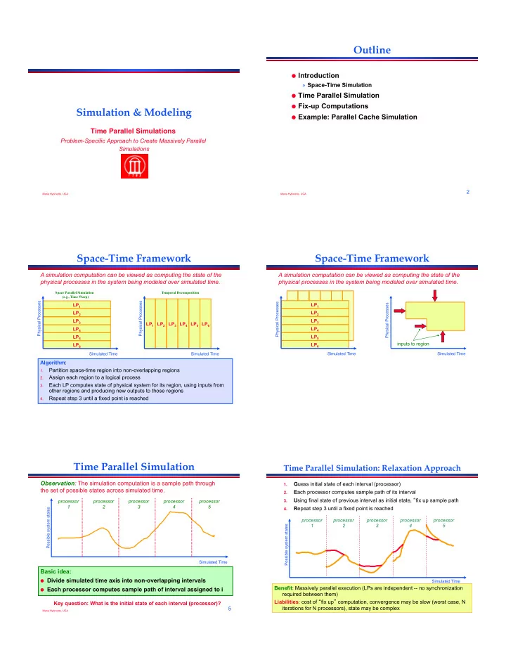
Space-Time Framework
A simulation computation can be viewed as computing the state of the physical processes in the system being modeled over simulated time.
LP1 LP6 LP5 LP4 LP3 LP2
Simulated Time Physical Processes
LP1 LP6 LP5 LP4 LP3 LP2
Simulated Time Physical Processes
Algorithm:
1.
Partition space-time region into non-overlapping regions
2.
Assign each region to a logical process
3.
Each LP computes state of physical system for its region, using inputs from
- ther regions and producing new outputs to those regions
4.
Repeat step 3 until a fixed point is reached
Space Parallel Simulation (e.g., Time Warp) Temporal Decomposition
Maria Hybinette, UGA
4
LP1 LP6 LP5 LP4 LP3 LP2
Space-Time Framework
A simulation computation can be viewed as computing the state of the physical processes in the system being modeled over simulated time.
Simulated Time Physical Processes
inputs to region LP1 LP6 LP5 LP4 LP3 LP2
Simulated Time Physical Processes
Maria Hybinette, UGA
5
Time Parallel Simulation
Basic idea:
- Divide simulated time axis into non-overlapping intervals
- Each processor computes sample path of interval assigned to i
Simulated Time Possible system states
Observation: The simulation computation is a sample path through the set of possible states across simulated time.
processor 1 processor 4 processor 3 processor 5 processor 2
Key question: What is the initial state of each interval (processor)?
Maria Hybinette, UGA
6
Time Parallel Simulation: Relaxation Approach
1.
Guess initial state of each interval (processor)
2.
Each processor computes sample path of its interval
3.
Using final state of previous interval as initial state, fix up sample path
4.
Repeat step 3 until a fixed point is reached
processor 1 processor 2 processor 3 processor 4 processor 5
Possible system states Simulated Time