Outline 1. Evaluation Functions 2. State-of-the-art game playing - - PDF document

SLIDE 1

1

1

CS 331: Artificial Intelligence Adversarial Search II

2

Outline

• 1. Evaluation Functions
• 2. State-of-the-art game playing programs
• 3. 2 player zero-sum finite stochastic games
• f perfect information

3

Evaluation Functions

4

Evaluation Functions

• Minimax and Alpha-Beta require us to search all

the way to the terminal states

• What if we can’t do this in a reasonable amount of

time?

• Cut off search earlier and apply a heuristic

evaluation function to states in the search

• Effectively turns non-terminal nodes into terminal

leaves

5

Evaluation Functions

• If at terminal state after cutting off search, return

actual utility

• If at non-terminal state after cutting off search,

return an estimate of the expected utility of the game from that state

T Cutoff

6

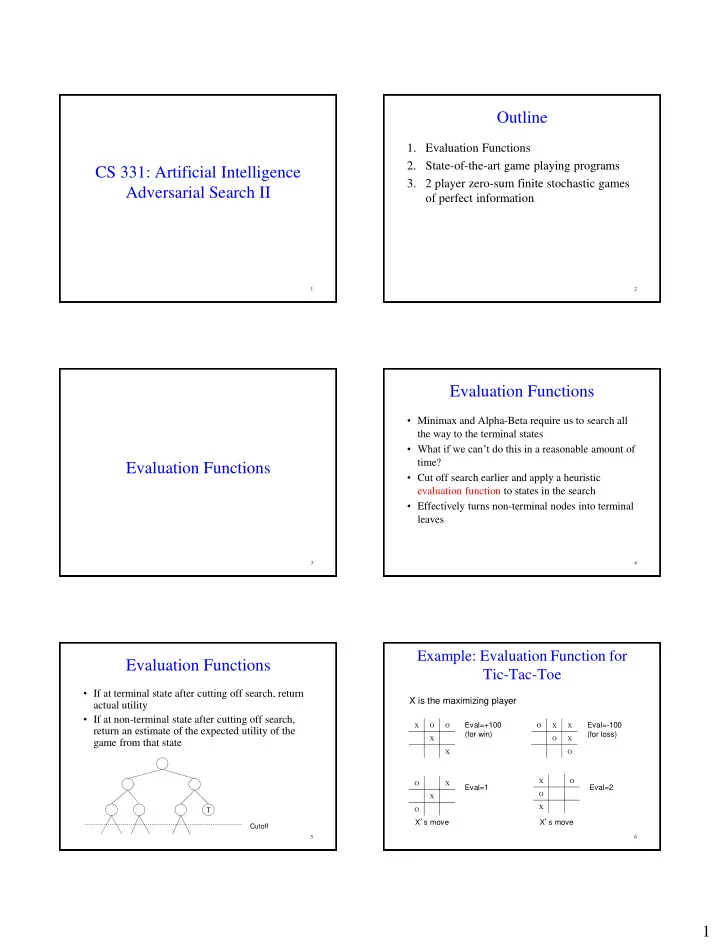
Example: Evaluation Function for Tic-Tac-Toe

X O O X X

Eval=+100 (for win)

O X X O

Eval=2 X’s move

O X X O X O

Eval=-100 (for loss)

X O O X

X’s move

X is the maximizing player

Eval=1

SLIDE 2

2

7

Properties of Good Evaluation Functions

1. Orders the terminal states in the same way as the utility function 2. Computation can’t take too long 3. Evaluation function should be strongly correlated with the actual chances of winning

Exact values don’t matter. It’s the ordering of terminal states that matters. In fact, behavior is preserved under any monotonic transformation of the evaluation function

8

Properties of Good Evaluation Functions

1. Orders the terminal states in the same way as the utility function 2. Computation can’t take too long 3. Evaluation function should be strongly correlated with the actual chances of winning

Even in a deterministic game like chess, the evaluation function introduces uncertainty because of the lack of computational resources (can’t see all the way to the terminal state so you have to make a guess as to how good your state is).

9

Coming up with Evaluation Functions

• Extract features from the game
• For example, what features from a game of

chess indicate that a state will likely lead to a win?





    

n i i i n n

s f w s f w s f w s f w s

1 2 2 1 1

) ( ) ( ) ( ) ( ) EVAL( 

Coming up with Evaluation Functions

Weighted linear function:

wi’s are weights fi’s are features of the game state (e.g. # of pawns in chess) The weights and features are ways of encoding human knowledge of game strategies into the adversarial search algorithm

11

Coming up with Evaluation Functions?

• Suppose we use the weighted linear

evaluation function for chess. What are two problems with it?

• 1. Assumes features are independent
• 2. Need to know if you’re at the beginning,

middle, or end of the game

12

Alpha-Beta with Eval Functions

Replace: if TERMINAL-TEST(state) then return UTILITY(state) With if CUTOFF-TEST(state,depth) then return EVAL(state) Also, need to pass depth parameter along and need to increment depth parameter with each recursive call.

SLIDE 3

3

13

The depth parameter

• CUTOFF-TEST(state,depth) returns:

– True for all terminal states – True for all depth greater than some fixed depth limit d

• How to pick d?

– Pick d so that agent can decide on move within some time limit

14

Quiescence Search

• Suppose the board at the

left is at the depth limit

• Black ahead by 2 pawns

and a knight

• Heuristic function says

Black is doing well

• But it can’t see one more

move ahead when White takes Black’s queen

15

Quiescence Search

• Evaluation function should only be applied

to quiescent positions

• i.e. positions that don’t exhibit wild swings

in value in the near future

• Quiescence search: nonquiescent positions

can be expanded further until quiescent positions are reached

16

Horizon Effect

• Stalling moves push an unavoidable and

damaging move by the opponent “over the search horizon” to a place where it cannot be detected

• Agent believes it has avoided the damaging,

inevitable move with these stalling moves

17

Horizon Effect Example

18

Singular Extensions

• Can be used to avoid horizon effect
• Expand only 1 move that is clearly better than all
• ther moves
• Goes beyond normal depth limit because

branching factor is 1

• In chess example, if Black’s checking moves and

White’s king moves are clearly better than the alternatives, then singular extension will expand search until it picks up the queening

SLIDE 4

4

19

Another Optimization: Forward Pruning

• Prune moves at a given node immediately
• Dangerous! Might prune away the best

move

• Best used in special situations e.g.

symmetric or equivalent moves

20

Chess

• Branching factor: 35 on average
• Minimax lookahead about 5 ply
• Humans lookahead about 6-8 plies
• Alpha-Beta lookahead about 10 plies

(roughly expert level of play)

If you do all the optimizations discussed so far

21

State-of-the-art Game Playing Programs

22

State of the Art Game Programs

• Checkers (Samuel, Chinook)
• Othello (Logistello)
• Backgammon (Tesauro’s TD-gammon)
• Go (AlphaGo – guest lecture Friday!)
• Bridge (Bridge Baron, GIB)
• Chess

23

Chess

• Deep Blue – Campbell, Hsu, Hoane
• 1997 – Deep Blue defeats Garry Kasparov

in a 6 game exhibition match

24

Chess

• Deep Blue Hardware:

– Parallel computer with 30 IBM RS/6000 processors running the software search – 480 custom VLSI chess processors that performed:

• Move generation (and move ordering)
• Hardware search for the last few levels of the tree
• Evaluation of leaf nodes

SLIDE 5

5

25

Chess

• Algorithm:

– Iterative-deepening alpha-beta search with a transposition table – Key to success: generating extensions beyond the depth limit for sufficiently interesting lines of forcing/forced moves – Reaches depth 14 routinely, depth 40 in some cases – Evaluation function:

• Had over 8000 features
• Used an opening of about 4000 positions
• Database of 700,000 grandmaster games
• Large endgame database of solved positions (all positions with

5 pieces, many with 6 pieces remaining)

26

Chess

• So was it the hardware or software that

made the difference?

– Campbell et al. say search extensions and evaluation function were critical – But recent algorithmic improvements allow programs running on standard PCs to beat

• pponents running on massively parallel

machines

27

2 player zero-sum finite stochastic games of perfect information

28

But First…A Mini-Tutorial on Expected Values

What is probability?

– The relative frequency with which an outcome would be obtained if the process were repeated a large number of times under similar conditions

Example: Probability of rolling a 1 on a fair dice is 1/6

29

Expected Values

• Suppose you have an event that can take a

finite number of outcomes

– E.g. Rolling a dice, you can get either 1, 2, 3, 4, 5, 6

• Expected value: What is the average value

you should get if you roll a fair dice?

30

Expected Values

What if your dice isn’t fair? Suppose your probabilities are:

Value Prob 1 2 3 4 5 6 1 Value Prob 1 0.5 2 3 4 5 6 0.5 Value Prob 1 0.1 2 0.1 3 0.2 4 0.2 5 0.3 6 0.1 OR OR

SLIDE 6

6

31

Expected Values

The expected value is a weighted average of the probability of an outcome times the value of that

• utcome



• me)

value(outc * me) Prob(outco

Value Prob 1 0.1 2 0.1 3 0.2 4 0.2 5 0.3 6 0.1

Expected Value = (0.1)(1)+(0.1)(2)+(0.2)(3)+(0.2)(4)+(0.3)(5)+(0.1)(6) = 0.1 + 0.2 + 0.6 + 0.8 + 1.5 + 0.6 = 3.8

32

2 player zero-sum finite stochastic games of perfect information

A B Chance Chance p=0.1

• 50

p=0.9 +10

• 2
• 12

+10 p=0.5 p=0.5

• Need to calculate expected value for

chance nodes

• Calculate expectiminimax value instead of

minimax value

MAX MIN

33

2 player zero-sum finite stochastic games of perfect information

A B Chance Chance p=0.1

• 50

p=0.9 +10

• 2
• 12

+10 p=0.5 p=0.5

(0.5)(10)+(0.5)(-12)=

• 1

MAX MIN

34

2 player zero-sum finite stochastic games of perfect information

A B Chance Chance p=0.1

• 50

p=0.9 +10

• 2
• 12

+10 p=0.5 p=0.5

(0.1)(-50)+(0.9)(10)=4 (0.5)(10)+(0.5)(-12)=

• 1
• 2

MAX MIN

35

2 player zero-sum finite stochastic games of perfect information

A B Chance Chance p=0.1

• 50

p=0.9 +10

• 2
• 12

+10 p=0.5 p=0.5

(0.1)(-50)+(0.9)(10)=4 (0.5)(10)+(0.5)(-12)=

• 1
• 2

4

MAX MIN

36

Expectiminimax

 ) IMAX( EXPECTIMIN n ) UTILITY(n ) IMAX( EXPECTIMIN max

) ( Successors s

s

n 

) IMAX( EXPECTIMIN min

) ( Successors s

s

n 







(n) Successors s

) IMAX( EXPECTIMIN ) ( s s P

If n is a MAX node If n is a terminal state If n is a chance node If n is a MIN node

SLIDE 7

7

37

Complexity of Expectiminimax

• Minimax – O(bm)
• Expectiminimax – O(bmnm)

n = # of possibilities at a chance node (assuming all chance nodes have the same number of possibilities)

Expectiminimax is computationally expensive so you can’t look ahead too far! The uncertainty due to randomness accounts for the expense.

CW: Expectiminimax

38

What is the expectiminimax value of the root node?

39

What you should know

• What evaluation functions are
• Problems with them like quiescence,

horizon effect

• How to calculate the expectiminimax value
• f a node