SLIDE 3
- u = [−L + 2 · l(u), −L] × [L + 2 · l(u), L], with L =
cos(π/mu), (x, y) are the coordinates of p, ψu(p) =
bu
j,k · Bm j (x) · Bn k (y)
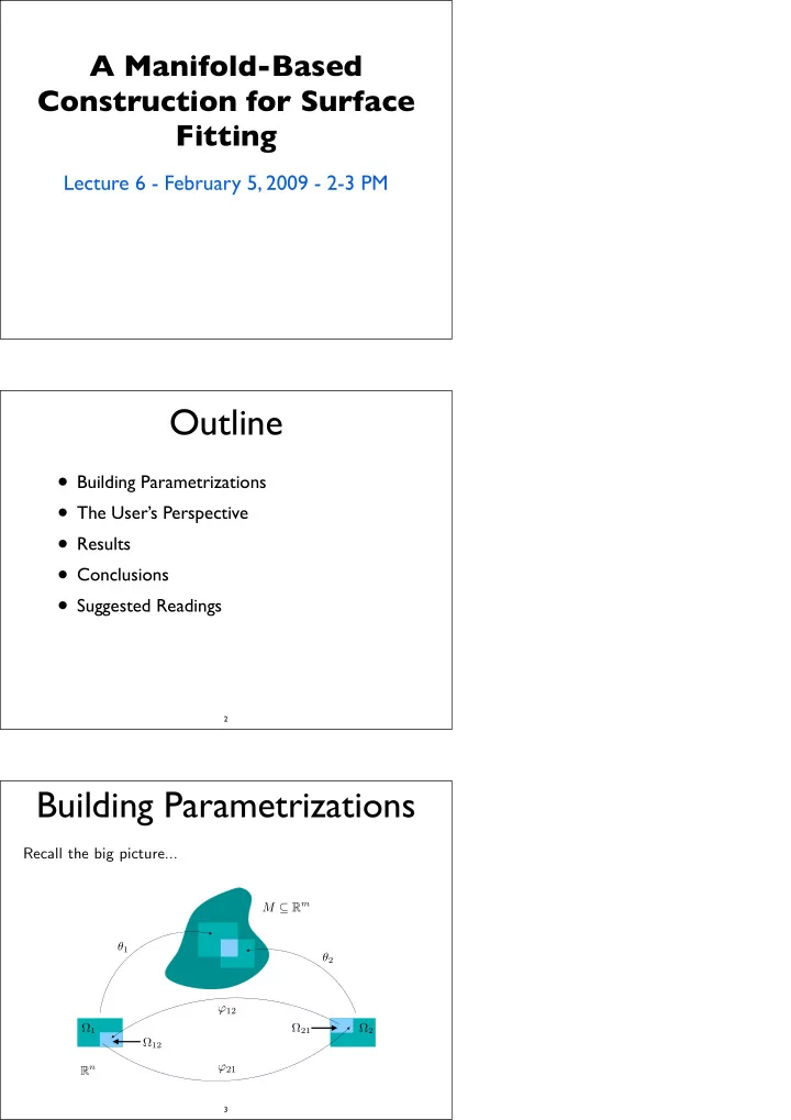
Building Parametrizations
Ωu
L = cos(π/mu) (2 · l(u), 0) [−L + 2 · l(u), −L] [L + 2 · l(u), −L] [L + 2 · l(u), L] [−L + 2 · l(u), L]
p = (x, y)
7
Building Parametrizations
j,k) ⊂ R3 are the control points, with 0 ≤ j ≤ m and
0 ≤ k ≤ n, R3
b0,0 b1,0 b2,0 b0,1 b1,1 b2,1 b0,2 b1,2 b2,2
Ex: m = 2 and n = 2
p1,0 p2,0 p0,1 p1,1 p2,1 p0,2 p1,2 p2,2 = (L + 2 · l(u), L) p0,0 = (−L + 2 · l(u), L)
R2 ψu(p) =
bu
j,k · Bm j (x) · Bn k (y)
8
Building Parametrizations
ψu(p) =
bu
j,k · Bm j (x) · Bn k (y)
Bl
i(t) =
l i
r − t r − s l−i · t − s r − s i is the i-th Bernstein polynomial of degree l over the affine frame [s, r], where [s, r] = [−L+2·l(u), L+2·l(u)] (or [s, r] = [−L, L]), for every i ∈ {0, . . . , l}. Note that Bl
i is a scalar function, and recall that the following
holds:
Bm
j (x) · Bn k (y) = 1, ∀x, y ∈ [0, 1] .
9