Outline Fine-Grain Register Allocation Based on a Global Spill - - PDF document

SLIDE 1

• Fine-Grain Register Allocation Based on a

Global Spill Costs Analysis

• 2003. 9. 25 (Thr.)

Seoul National University

Dae-Hwan Kim dhkim@capp.snu.ac.kr Hyuk-Jae Lee hjlee@ee.snu.ac.kr

Outline

q

Graph coloring register allocation

q

Motivation example

q

Proposed register allocation algorithm

q

Allocation benefit model

q

Experimental results

q

Conclusions

Overview of Register Allocation

q

Determines whether a live range (variable/temporary) is to be stored in a register or in memory

q

Goal:

• Store live ranges as many as possible in registers
• Minimize the number of memory accesses (load/store instructions)

q

An important compiler technique

• The reduction of load/store instructions leads to the decrease of execution

time, code size and power consumption.

Graph-Coloring Register Allocation

q

Dominant allocation paradigm (Chaitin, Brigss, …)

q

Models register allocation problem as a graph coloring problem

• f an interference graph

q

Interference graph: an undirected graph, where

• A node: a live range
• there is an edge between two nodes if corresponding live ranges interfere.
• Interfering live ranges can not share the same register

q

The contribution of graph coloring approach: the simplicity by abstracting each live range as a single node of an interference graph

Graph-Coloring Limitations

q

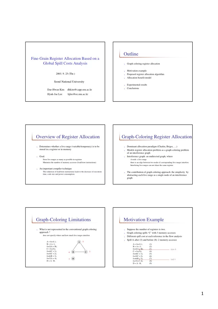
What is not represented in the conventional graph coloring approach ?

• does not specify where and how much live ranges interfere

A = foo1( ); B = A + 1; foo2(A + B); C = foo3(); foo4(C + 1); foo5(C + 2); foo6(B + 3); foo7(A + 4); D = A - B;

A B C D

5 4 3 1

Motivation Example

q

Suppose the number of registers is two.

q

Graph coloring spills ‘C’ with 3 memory accesses

q

Different spill cost at each reference in the flow analysis

q

Spill A after (3) and before (8): 2 memory accesses

A = foo1( ); (1) B = A + 1; (2) foo2(A + B); (3) C = foo3(); (4) foo4(C + 1); (5) foo5(C + 2); (6) foo6(B + 3); (7) foo7(A + 4); (8) D = A - B; (9)

SLIDE 2

• Overview of Proposed Algorithm

q

Decides whether to allocate a register or not for every reference

• f a variable

q

When there is no free register, it determines allocation based on the allocation benefit in the reference flow

q

Two stages

• Variable allocation: variables are allocated with the number of machine

registers

• Scratch allocation: temporaries and unallocated variables are allocated

Variable Reference Flow Graph

q

The proposed approach constructs a varef-graph (variable reference flow graph)

q

Node: a variable reference

q

Edge: control flow of the program (i.e, execution order of the variable references of the program)

q

The varef-graph models the execution order of the references in the program.

Varef-Gaph Example

(1) A = 1; (2) if (A) (3) B = 1; else (4) B = 2; (5) return A + B;

code example Variable reference flow graph

A A B B A B

1 2 3 4 5 6

Allocation Algorithm

q

The proposed algorithm visits each node of a varef-graph in the breadth-first order.

q

When no register is free for a node, the allocator estimates the benefit and loss of register preemption for each register, and selects the register with the maximum benefit.

q

If all registers have larger loss than benefit, no register is assigned to the node.

q

For those nodes that are not assigned to a register, the second stage register allocation, called scratch allocation, is performed.

Variable Allocation Algorithm

Any register available ?

Continue until all nodes visited Visit each node in the graph Assign the register with the maximum non-negative benefit Assign any register Assign the previously assigned register

Previously assigned register available ?

No Yes Yes No

Register Allocation Benefit

q

BenefitRegAlloc(n,r) = PenaltySpill(n,r) – PenaltyPreempt(n,r)

• n: node number, r: register number

q

PenaltySpill(n,r): the total number of load/store instructions that are required if node ‘n’ is spilled.

q

PenaltyPreempt(n,r): the total number of load/store instructions that are required when node ‘n’ preempts register ‘r’.

SLIDE 3

• Impact Range

q

The decision for one node affects the register allocation for another node

• If node ‘1’ is spilled, node ‘6’ is also spilled

q

Impact Range: the set of the nodes that are affected by the register allocation for a given node.

q

The impact range of node ‘n’ for register ‘r’ is defined as the path from node ‘n’ to the next references of a variable that currently holds register ‘r’.

A =

1 2

B =

4

C = C =

3 5

= C

6

= A

Impact Range Example (1)

q Suppose register allocation visits node ‘5’ q Suppose the number of registers is 2

q VarHold(n,r): the variable that holds register ‘r’ when

the register allocation is performed for node ‘n’.

q NodeHold(n,r): the nodes for VarHold(n,r)

q VarHold(5,r1)=‘A’, NodeHold(5, r1) = {1,2}. q NextRef(n) = {p| p is a next reference of n} . q NextRef(1) = {11} , NextRef(2) = {8,9,11}, q NextRef({1,2}) = {8, 9,11} q ImpactRange(5,r1) = path (5, 8) ∪ path (5, 9) ∪ path (5,11)

= { } ∪ { } ∪ path(5,11) = {5, 7, 10, 11} A

1 3 5 7 10

B N N C A

2 4 6 8 9

B B A A R1 R2 R1 R2

11

A

Impact Range Example (2)

q subpath(n,p,s) is the path(p,s) ⊂ path(n,s). q subpath(1, 5, 11) = path(5, 11) = {5, 7, 10, 11} q SubPathRange (n,p) = ∪s subpath (n, p, s)

for all s ∈NextRef(n)

q SubPathRange (S,p) = ∪n SubPathRange (n, p) for all n ∈ S q ImpactRange(n,r) = SubPathRange (NodeHold(n,r),n) q ImpactRange(5, ‘r1’)

= SubPathRange(NodeHold(5,r1), 5) = SubPathRange({1,2}, 5) = subpath(1, 5, 11) ∪ subpath(2, 5, 8) ∪ subpath(2, 5, 9) ∪ subpath(2, 5, 11) = {5, 7, 10,11 } ∪ { } ∪ { } ∪ {5, 7, 10.11} = {5, 7, 10,11} A

1 3 5 7 10

B N N C A

2 4 6 8 9

B B A A R1 R2 R1 R2

11

A

Definition of Impact Set

q

Only two types of nodes in the impact range contribute to BenefitRegAlloc(n,r) 1) The node that references the same variable as node ‘n’ 2) The node that references the variable that holds register ‘r’ when node ‘n’ is visited for register allocation.

q

var(n): the variable that is referenced by node ‘n’.

q

VarHold(n,r): the variable that holds register ‘r’ when the register allocation is performed for node ‘n’

q

ImpactSet(n,r) = { m| m ∈ ImpactRange(n,r), and (var(m) = var(n) or var(m) = VarHold(n,r)}

Impact Set Example

q ImpactRange(5,r1) = path (5, 8) ∪ path (5, 9) ∪

path (5,11) = { } ∪ { } ∪ path(5,11) = {5, 7, 10, 11}

q var(5) = ‘N’ q VarHold(5, ‘r1’) = ‘A’ q ImpactSet(5, ‘r1’) = { 5, 7, 11}

A

1 3 5 7 10

B N N C A

2 4 6 8 9

B B A A R1 R2 R1 R2

11

A

Benefit Model

q

PenaltySpill(n,r) = Σm∈ ImpactSet(n,r) and var(m)=var(n) cost(m)

q

PenaltyPreempt(n,r) = Σm∈ ImpactSet(n,r) and var(m)=VarHold(n,r) cost(m)

• n: node number, r: register number
• var(n): the variable that is referenced by node ‘n’.
• VarHold(n,r): the variable that holds register ‘r’ when the register

allocation is performed for node ‘n’.

q

BenefitRegAlloc(n,r) = PenaltySpill(n,r) – PenaltyPreempt(n,r)

• n: node number, r: register number

SLIDE 4

• Cost of a Node

q

Let NodeCost(n) be the cost of the execution of ‘n’

q

NodeCost(n) = 10d where d is a loop depth of a node n’.

q

Consider the cost of ‘2’ for ‘r1’

q

ImpactSet(2, ‘r1’) = { 2, 5}

q

Node ‘6’ is not in the impact set, however, it is affected by the allocation of node ‘2’

q

cost(2) = NodeCost(2) + NodeCost(6)

q

cost(m) |m:definition = NodeCost(m) + Σ k ∈ NextRef(m), k:use, k ∉ impact set NodeCost(k)

q

cost(m) |m:use= NodeCost(m) + Σ k ∈ PrevRef(m), k ∉ impact set NodeCost(k) A =

1 2

B =

4

C = C =

3 5

= A

6

= B R1

Benefit Estimation Example

A = B = A = B = = B = A = B

1 2

BenefitRegAlloc(2, R1) = PenaltySpill(2, R1) - PenaltyPreempt(2,R1)

5 6 7

ImpactSet(2, R1) = {2, 3, 4, 5, 6} PenaltySpill(2, R1) = cost(2) + cost(3) + cost(5) = NodeCost(2) + NodeCost(3) + NodeCost(5) + NodeCost(7) = 4 PenaltyPreempt(2, R1) = cost(4) + cost(6) = NodeCost(1) + NodeCost(4) +NodeCost(6) = 3 BenefitRegAlloc(2, R1) = 4 –3 = 1

3 4

R1

Scratch Allocation

q

Unallocated variables and temporaries are allocated.

q

Nodes corresponding to temporaries are added to the varef-graph.

q

PenaltyPreempt(s,r) = Σm∈ ImpactRange(s,r) and var(m)=VarHold(n,r) cost(m)

q

PenaltySpill(s,r) = Σm∈ ImpactRange(s,r), m∈ CLASS(s) cost(m)

q

If a scratch ‘s’ preempts a register ‘r’, then this register can be used for the scratch ‘s’ as well as other scratches that are in the impact range.

q

However, not all the scratches in the impact range can be allocated to the same register, due to the overlapping of their live ranges.

q

CLASS(s): the class that the scratch ‘s’ belongs to so that all scratches in the class can be allocated to the same register.

Derivation of Class

q

All the scratches are colored with infinite colors.

q

Scratches are partitioned into classes according to the assigned color.

q

Example

• two classes: {t1, t3, t5} and {t2, t4, t6}

a = t1 + t2 t5 = t3- t4 b = t5 - t6 a = C1 + C2 C1 = C1- C2 b = C1 - C2

Allocation Example (1)

ImpactRange(t1, R1) = {t1, t2, t3, t4, t5, 3} PenaltySpill(t1, R1) = cost(t1) + cost(t3) + cost(t5) = 3 PenaltyPreempt(t1, R1) = cost(3) = NodeCost(1) + NodeCost(3) = 2 BenefitRegAlloc(t1, R1) = 3 –2 = 1 Assume two registers. At node ‘t1’, runs out of registers

A = B = 1 2

R1 R2 t1 C1 t2 C2 t3 C1 t4 C2 t5 C1

= A t6 3

t7 C1 = B C2

4

R1 R2

Allocation Example (2)

PenaltySpill(t1, R2) = NodeCost(t1) + NodeCost(t3) + NodeCost(t5) + NodeCost(t6) = 4 PenaltyPreempt(t1, R2) = cost(4) = NodeCost(2) + NodeCost(4) = 11 BenefitRegAlloc(t1, R2) = 4–11 = -7 ‘t1’ preempts register ‘R1’, and ‘t1’, ‘t3’, and ‘t5’ are assigned to ‘R1’. BenefitRegAlloc(t1, R1) = 3 –2 = 1 ImpactRange(t1, R2) = {t1, t2, t3, t4, t5, 3, t6, t7,4}

A = B = 1 2

R1 R2 t1 C1 t2 C2 t3 C1 t4 C2 t5 C1

= A t6 3

t7 C1 = B C2

4

R1 R2

SLIDE 5

• Experimental Results

q

Implemented in LCC targeting ARM7TDMI

q

With the eight benchmarks, an average of 34.3% improvement is achieved over the graph coloring approach

Reduction Ratio(%) 10 20 30 40 50 60 70 80

g721 yacc mpeg adpcm cpp pgp gsm runlength average

Reg: 4 Reg: 8 Reg: 12

Compilation Time Measurements

benchmark Number of registers 4 8 12 g721

1.64 1.86 1.97

yacc

1.73 2.13 2.01

mpeg

3.28 2.77 2.79

adpcm

1.29 1.49 1.62

rep

2.21 2.00 2.17

pgp

1.42 1.75 1.67

gsm

1.49 1.24 1.10

runlengt

1.34 1.41 1.93

On average, 1.85 times larger than that for Briggs’ allocator.

Complexity Analysis

q

The dominant complexity: the derivation of the impact range

q

N: the number of nodes in the varef-graph

q

The derivation of the impact range of a node for a register: O(N)

q

Iterated N times for each node ;

q

Total Complexity: O(N2)

q

In practice, the next reference of a variable is generally located close to the node, thus search spaces are localized.

Conclusions

q

Improves the Briggs’ allocator by an average of 34.3%

q

The compilation time increase by the amount of 85%

q

Time overhead is not serious considering that graph-coloring allocators run fast in practice.

q

The proposed varef-graph can be used for further optimizations such as instruction scheduling