Outline of the lecture Outline of the lecture Inequality and income - - PowerPoint PPT Presentation

Inequality and Development – Week 10 March 12

Readings: Ray chapter 7 Ray chapter 7 Benabou & Mookherjee chapter 4 and 12

1

Questions that we will discuss today

T k hi i ll i i i i l di ib i f b h

• Take historically given an initial distribution of assets, but then

ask the question:  Do inequalities worsen or narrow with economic development?  How are aggregates, such as income, wealth, savings, and growth rates affected by inequality?  In turn, how do these variables affect the evolution of inequality?

2

Outline of the lecture Outline of the lecture

E i i l tt b t i lit d i d l t/i  Empirical pattern between inequality and economic development/income.  The inverted-U hypothesis  From inequality to aggregates  Inequality → savings.  Inequality → growth Inequality → growth.  Inequality → credit constraints.  Inequality → occupational choice.

Inequality → savings → Inequality Inequality → credit constraints → Inequality Inequality → occupational choice → Inequality Inequality → growth → Inequality

 From aggregates to inequality  Savings → Inequality  Growth → Inequality.  Credit constraints → Inequality.  Occupational choice → Inequality. p q y

3

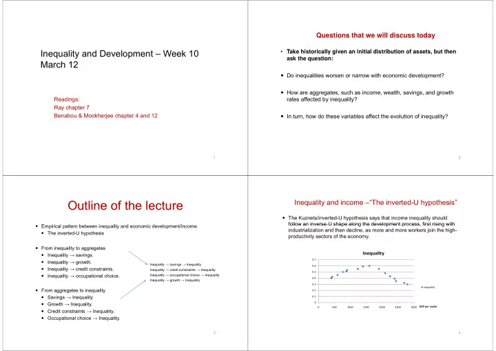
Inequality and income –“The inverted-U hypothesis” q y yp

 The Kuznets/inverted-U hypothesis says that income inequality should follow an inverse-U shape along the development process first rising with follow an inverse U shape along the development process, first rising with industrialization and then decline, as more and more workers join the high- productivity sectors of the economy.

0.7

Inequality

0.4 0.5 0.6 0.1 0.2 0.3 inequality 500 1000 1500 2000 2500 3000 GDP per capita

4

Income and inequality: Uneven and compensatory changes Income and inequality: Uneven and compensatory changes

Wh i i i i i h

• When a country experience an increase in per capita income, the

change might stem roughly from three sources. 1. Steady sequence of annual growth. 2. Uneven change 3 Compensatory change 3. Compensatory change

• Inverted-U: Uneven changes occur at low levels of income, whereas

g , compensatory changes occur at higher levels of income.

5

First uneven, then compensatory? , p y

1. Economic development: Large transfers of people from relatively poor to relatively advanced sectors of the economy advanced sectors of the economy. 2. Technical progress initially benefits the (relatively) small industrial sector. Technical progress is likely to have a more uneven character at low levels of income progress is likely to have a more uneven character at low levels of income. 3. Technical progress is initially biased against unskilled labor and tends to drive down these wages. these wages. 4. Industrialization brings profits to a minority that possess the financial endowments and entrepreneurial drive to take advantage of the new opportunities that open up. p g pp p p 5. These gains ultimately find their way to everybody, as the increased demand for labor drives up wages.

6

Why did Kuznets suggest an inverted-U? y gg

 Observed inequality decline in the United States between 1913 and 1948 1948.  No data prior to the creation of the federal income tax in 1913, but the general presumption was that inequality had been rising during the nineteenth century.  Kuznets used the ratio of the income share of the richest 20% of the population to that of the poorest 60% of the population.  Kuznets (1963):

 Eighteen countries Eighteen countries  The income shares of upper income groups in developed countries where lower than in poorer developing countries, and highest in middle income countries.

7

Testing the inverted U hypothesis Testing the inverted-U hypothesis  There are two ways to test the inverted-U:

1. Cross-section study: examine variations in inequalities across countries that are at different stages in the development process. 2. Study an individual country over time and note the resulting changes in inequality that occurs with development.

8

An inverted U in the cross section? An inverted-U in the cross section?

P k t (1973) Paukert (1973): 56 countries were classified into different income categories according to their per capita GDP in 1965, in U.S dollars.

Income category Average Gini Range of Gini Less than 100 0.419 0.33‐0.51 101‐200 0.468 0.26‐0.50 201‐300 4.499 0.36‐0.62 301‐500 0.494 0.30‐0.64 501‐1000 0.438 0.38‐0.58 1001 2000 0 401 0 30 0 50 1001‐2000 0.401 0.30‐0.50 2001 and higher 0.365 0.34‐0.39

9

An inverted U in the cross section? An inverted-U in the cross section?

• The table reveals two things:

1 Fi t th t b l ti hi b t i lit 1. First, there appears to be a relationship between inequality and GDP of the kind predicted by Kuznets. 2. Second, that the variation within a particular category is high.

10 11

An inverted-U in the cross section?

• Ahluwalia (1976) analyzed a sample of sixty countries: 40

Ahluwalia (1976) analyzed a sample of sixty countries: 40 developing, fourteen developed, and six socialist.

• The population of each country is divided into quintiles.
• For each quintile we have the following regression:

S A b

2 D

• Si=A+byi+cyi

2+Di+errori

12

An inverted-U in the cross section

• Si=Ai+byi+cyi

2+Di+errori

Income share Constant y y2 Socialist R2 Top 20% ‐57.58* 89.95* ‐17.56* ‐20.15* 0.58 Middle 40% 87.03* ‐45.59* 9.25* 8.31* 0.47 L t 20% 27 31* 16 97* 3 06* 5 54* 0 54 Lowest 20% 27.31* ‐16.97* 3.06* 5.54* 0.54

• For all quintiles but the highest, income shares tends to fall initially

with a rise in per capita GNP and then rises beyond a certain point.

• There seems to be an inverted-U in the cross section, or is there?

13

Inverted U ”Words of Caution” Inverted-U Words of Caution

• The data exhibit too much variation to support some law of
• The data exhibit too much variation to support some law of

economic change.

• A regression of the form estimated in the example is not the only

functional form that can deliver an inverted U shape functional form that can deliver an inverted-U shape.

• The inverted-U is, to some extent, an artifact of the statistical

methodology that is used in inequality measurement (see next page)

14

Initially all five groups have 100. What happens if one after one get an adittional 100?

90 100

pp g

60 70 80

• me

40 50 60 Cumulative Inco all same income 10 20 30 1 with 200 2 with 200 3 with 200 4 with 200 10 10 20 30 40 50 60 70 80 90 100 Cumulative Population p

15

Inverted-U ”Words of Caution”

• A deep problem with cross-sectional studies: Implicit assumption

that all countries have the same inequality income relationship that all countries have the same inequality-income relationship.

• Not only are we to believe that they follow the same qualitative

pattern, but the same quantitative pattern as well – the income- inequality curve is the same curve for all countries inequality curve is the same curve for all countries.

• The opposite extreme is to say that every country is completely

different: one country might have one sort of curve and the other might have another and there is no relationship between the two might have another, and there is no relationship between the two.

16

Inverted-U ”Words of Caution” Inverted U Words of Caution

• Suppose that income affects inequality in the same way across
• Suppose that income affects inequality in the same way across

countries, so that b and c are all the same, but that some countries have some separate structural reason for higher or lower inequality.

• This is the same as saying that the curves (by country) are all

parallel to one another, but we allow for different intercept terms. parallel to one another, but we allow for different intercept terms.

17

A “L ti ff t”? A “Latin effect”?

• Is the inverted-U that we see in the cross section driven by the
• bservation

a) that middle-income countries have high inequality. b)

• r that middle-income countries are largely Latin American and

b)

• r that middle income countries are largely Latin American and

that Latin American countries have higher inequalities for other, structural reasons.

18

.4

Latin American

.3 .2 .1 500 1000 1500 2000 2500 y % C 95% CI Fitted values ineq

19

A “Latin effect”? A Latin effect ?

• One sensible way to check whether this makes sense is to put in a

dummy variable for Latin American countries in the regression. Th ti t d ffi i t th d th b i t t d

• The estimated coefficient on the dummy can then be interpreted as

the “importance” as far as inequality is concerned of being Latin American.

20

.5 .4 .3 .2 .1 500 1000 1500 2000 2500 y 95% CI Fitted values 95% CI Fitted values ineq ineq 21

Country Fixed Effect y

• Once we open the door to the inclusion of a Latin dummy we

Once we open the door to the inclusion of a Latin dummy, we might as well try out dummies for each continent or each different country in the sample.

• This allows us to make use of a combined data set or panel,

which can be used to estimate the common coefficients b and c which can be used to estimate the common coefficients b and c more precisely.

22

What happens if country-specific dummies are used for the intercept term Ai?

• Deninger and Squire (1996)

Deninger and Squire (1996)

– The Kuznets inverted U hypothesis largely vanishes. – The coefficients b and c have the wrong signs for an inverted-U, and the coefficients where not significant. coefficients where not significant.

• This suggests that structural differences across countries or regions

t th ill i f i t d U h i d d th i may create the illusion of an inverted-U, when indeed there is no such relationship.

• When countries are examined separately, there is some evidence of

an inverted-U, but also some evidence of an direct U and some evidence that inequality falls with income evidence that inequality falls with income.

23

Was Kuznets wrong? An inverted U within countries? Was Kuznets wrong? An inverted-U within countries?

• With panel-cross-country data we fail to replicate an inverted-U

when country or regional fixed effects are taken into account.

• If would be misleading however to conclude that Kuznets
• If would be misleading, however, to conclude that Kuznets

hypothesis is no longer of interest.

• A number of poor countries may not have passed what Kuznets

identified as the initial industrialization stage identified as the initial industrialization stage.

24

Was Kuznets wrong? An inverted-U within countries?

• Important pieces of evidence was missing to the Kuznets (1954)
• Important pieces of evidence was missing to the Kuznets (1954)
• ptimistic interpretation of what happened to the developed

world.

• Because existing data at the time ended in 1948, Kuznets was

not able to see that the inequality decline in the United States not able to see that the inequality decline in the United States and in most other developed countries stopped almost immediately after World War II.

• Available US data did not allow him to decompose income

inequality trends into labor income and capital income. q y p

25 26

Was Kuznets wrong? An inverted U within countries? Was Kuznets wrong? An inverted-U within countries?

• Although top income shares declined substantially in France
• ver the period 1900-1950, wage inequality – as measured by

top wage shares remained extremely stable top wage shares remained extremely stable.

• The decline in income inequality was for the most part a capital

q y p p income phenomenon. Th f t th t it l h k l d th l di l d i th

• The fact that capital shocks played the leading role during the

1914-1945 period obviously does not imply that the technical change view of inequality dynamics has no relevance.

27

Top CEO incomes in the US Top CEO incomes in the US

28

Inequality and savings q y g

– We will start with “Inequality → savings” – Is inequality good or bad for saving?

Economy 1 A teacher with an income of 400,000 , A student with an income of 100,000 E 2 Economy 2 Two research assistants each with an yearly income of 250,000

• What is the effects on overall savings rates from going from

economy 1 to economy 2?

29

savings income

100,000 400,000 30

• Increasing marginal savings rates

savings

From this figure, we have that a reduction in inequality will reduce the volume of savings in the economy.

income

100,000 400,000 250,000 31

• Decreasing marginal savings rates

savings

From this figure, we have that a reduction in inequality will increase the volume of savings in the economy. in the economy.

income

100,000 400,000 250,000 32

How does savings change with income? How does savings change with income?

• There are several factors to be considered

There are several factors to be considered before we can come to a final judgment of this question question. S b i t d

• Subsistence needs
• Conspicuous consumption
• Aspiration and savings
• What emerges from this is not a clean picture.

33

• Savings and income: A more detailed view.

savings income

34

Inequality and savings Inequality and savings

• Effect of inequality on savings and growth

Effect of inequality on savings and growth.

– In an extremely poor country, redistribution may bring down the rate of savings and therefore the rate of growth in the medium or even long run run. – Without redistribution, there is a fraction of the population who possess the desire and the means to accumulate wealth. With redistribution, no person saves anything of any significance.

• Effect of savings and income to the evolution of

inequality. inequality.

– For many groups in society, there is a substantial difference between their notions of a desired standard of living and their actual standard of living and this might have an effect on savings behavior living, and this might have an effect on savings behavior.

35

Savings behavior as individual income drops below the income deemed necessary to achieve the desired standard of living.

As the shortfall increases, aspirations are created, which initially raises f f

Savings rate

the rate of savings for such income groups. As the shortfall continues to increase, poorer groups find that a high savings rate is simply too costly on their much-needed current consumption, and the savings rate starts to fall, making them fall

rate

p , g , g further behind the rich. The relatively poor might find themselves in a self-sustaining low- income trap, whereas the middle class grows more rapidly than either rich or poor rich or poor. We might observe high mobility between rich and middle-income groups, while a wall builds up between these groups and the poor.

Shortfall

Rich Poor Middle Class 36

Inequality, political redistribution, and growth q y, p , g

• Alesia and Rodric (1994), Perrson and Tabellini (1994):
• High economic inequality might retard economic growth by setting

up political demands for redistribution.

• Redistribution might take one of two broad forms:

1. Redistribute existing wealth among the broader population.

– Land reforms, confiscatory taxes on wealth. , y

2. Tax increments to the stock of wealth, rather than the existing lth b wealth base.

– These taxes, imposed on the margin, tend to bring down the rate of investment and therefore the rate of economic growth.

37

Point A is the pre-tax situation.

Consumption Tomorrow

Suppose that a tax is imposed on the return to investment. This has the effect of swiveling the rate-of-return line downward. Point B is now the post tax situation.

A

Now consider a lump-sum tax on this individual that pulls him down to exactly the same indifference curve.

B C

The tax on the rate of return reduces savings relative to the lump-sum tax.

B Consumption Today 38

Inequality, political redistribution, and growth Inequality, political redistribution, and growth

• Both lump-sum taxes and income taxes have income

effects that tend to reduce consumption effects that tend to reduce consumption.

• The income (investment) tax has an additional “price

( ) p effect” that tends to lower the rate of saving and investment.

• High levels of inequality may retard economic growth,

because such inequalities create a political demand for redistribution that can only be met by imposing taxes on increments to wealth, and not existing wealth.

• Such taxes may reduce the incentive to accumulate

wealth, and therefore the rate of economic growth.

39

Inequality and growth: Evidence Inequality and growth: Evidence

• Does initial inequality retard growth?
• Does initial inequality retard growth?
• The use of contemporaneous data on inequality and growth is not

p q y g very meaningful because we run into severe problems of endogeneity.

• We need data on inequality at the start of a relatively long period,

followed by growth figures for the subsequent period.

• What is a good proxy for initial inequality?

40

Inequality and growth: Evidence Inequality and growth: Evidence

O f l h i li i h i li f i h

• One proxy for wealth inequality is the inequality of income at that

time, but we must recognize that this is an imperfect proxy.

• Another proxy for wealth inequality is the inequality in some easy-to-

b t h l d

• bserve asset, such as land.
• Land inequality can only be a good proxy for overall inequality in

wealth if agriculture is either significantly important in the economy, h b f i ifi t i t i th t t

• r has been of significant importance in the recent past.

41

Initial inequality and subsequent growth Initial inequality and subsequent growth.

Alesina and Rodrik (1994)

Effect on per capita growth, 1960‐85 (1) (2) (3) Constant 6.22 (4.69) 6.24 (4.63) 6.21 (4.61) GDP60 ‐0.38 (3.25) ‐0.39 (3.06) ‐0.38 (2.95) Prim60 2.66 (2.66) 2.62 (2.53) 2.65 (2.56) Gini60 ‐3.47 (1.82) ‐3.45 (1.79) ‐3.47 (1.80) LandGini 5 23 (4 38) 5 24 (4 32) 5 21 (4 19) LandGini ‐5.23 (4.38) ‐5.24 (4.32) ‐5.21 (4.19) Dem*LGini 0.12 (0.12) Dem 0.02 (0.05)

42

Inequality, capital markets and development Th bl f ll t l – The problem of collateral

• What you have as collateral determines the degree to which you have

access to the credit market access to the credit market.

• In unequal societies, the poor may lack access to credit markets for

i l th th t th l k ll t l precisely the reason that they lack collateral.

• To the extent that credit is necessary to

a) Start a business b) Educate oneself or one’s children c) By inputs so that you can rent land and farm if d) Smooth out consumption expenditures in a fluctuation environment,

the poor are shut out from these markets, and everything else that credit can nourish.

43

Collateral – an example Collateral – an example

• The investment required to start up the business is $200,000.
• The business will hire fifty workers, who will be paid $5,000 each, and

produce and sell for a total revenue of $500 000 →profit 250 000 produce and sell for a total revenue of $500,000 →profit 250,000

• The lifetime of the business is one year. After this, the loan must be
• repaid. The interest rate on the loan is 10%.
• If I do not repay my loan, then my assets will be seized by the bank.
• There is also a 50-50 chance that I will be caught in which case I will
• There is also a 50-50 chance that I will be caught, in which case I will

go to jail (monetary equivalent $50,000) and the business profits for that year will be confiscated (cost $125,000).

44

Economic considerations underlying default - Economic considerations underlying default Collateral $100,000

Items If I pay If I default Direct payment 220,000 Direct payment 220,000 Collateral loss 110,000 Jail 50,000 , Seizure of profits 125,000 Total 220,000 285,000 , ,

45

Economic considerations underlying default - Collateral $20,000

Items If I pay If I default Direct payment 220,000 Collateral loss 22,000 Jail 50,000 Seizure of profits 125 000

Th b i i t i th t dit k t i ht b h t d f

Seizure of profits 125,000 Total 220,000 197,000

• The basic point is that credit markets might be shut down for

individuals who have relatively small amounts of collateral.

• This is because these individuals cannot credibly convince their

creditors that they will not default on their dept obligations.

46

Occupational choice and the credit constraint Occupational choice and the credit constraint

• Consider a very simple economy, with just three occupations:

y p y j p

• 1. Subsistence producer
• 2. Industrial worker

3 Entrepreneur

• 3. Entrepreneur
• Subsistence producers can produce some fixed amount z with

p p their labor. An ind strial

• rker can earn a

age

• An industrial worker can earn a wage w.
• An entrepreneur runs the sort of business that hires industrial

An entrepreneur runs the sort of business that hires industrial workers, but the business requires startup capital, I.

47

Occupational choice and the credit constraint Occupational choice and the credit constraint

• The profit in the business is equal to q – wm.

p q q

• If the loan is repaid at interest rate r, then net profit is equal to:

(q-wm) – (1+r)I

• The expected cost of default is some fine F, and a fraction γ of

the profits.

• With this information we can easily figure out whether a person
• With this information, we can easily figure out whether a person

with some given starting wealth W will be granted a loan.

48

Occupational choice and the credit constraint Occupational choice and the credit constraint

• You will honor the loan if

(**)

• This inequality tells us that banks will only give a loan to an

individual whose initial wealth is “high enough”.

49

Occupational choice and the credit constraint Occupational choice and the credit constraint

• The starting distribution of wealth gives us the following information:

It t ll th f ti f th l ti th t i h t t f – It tells us the fraction of the population that is shut out of entrepreneurship. – For each w, (**) tells us the minimum wealth level (W) that is required to have access to credit. – The higher the wage rate, the higher is the fraction of the population that is shut out of entrepreneurship. – The individuals who are shut out must choose between subsistence and market labor, and the choice depends on the wage rate.

50

Wage rates and fractions of people lacking access to credit

Wealth cutoff at a High wage Wealth cutoff at a Low wage nt Wealths (%) lation at Differen Popul Wealth Levels 51

Wage rates and fractions of people lacking access to credit g p p g

Fraction Lacking Access to Credit

1 Wage Rates 52

The supply curve of labor

Wages less than z will cause zero participation in the labor market. At w=z, there is a jump in labor supply. For higher wages, the labor supply steadily increases, as more and more people get shut

Wage rate

, p p g

• ut of entrepreneurship and must switch their
• ccupational choice to labor.

This process continues until we reach a high

rate w

p g enough wage, call it w such that the profits from running a business becomes exactly the same as labor income.

z

After this point everyone will jump into the labor market. If wages exceeds w, labor income exceeds

Labor

g , profit income, so no one will want to be an entrepreneur.

53

The demand curve of labor The demand curve of labor

• Start with a high wage that exceeds
• w. At such wages there is no demand

for labor at all, because no one wants to be an entrepreneur. Moving down to w we see a sudden jump in the demand for labor as people now enter entrepreneurship enter entrepreneurship.

• As the wage falls the demand for

w

• As the wage falls, the demand for

labor steadily rises, capturing the fact that more individuals have access to the credit market with lower wages.

Labor 54

Determination of equilibrium wage rate

If inequality is high (or the economy poor), so that are a large number of individuals with very low wealth, the equilibrium wage is z. For the lucky few who are originally wealthy (can become entrepreneurs) profits (and so income and wealth) are high wealthy (can become entrepreneurs), profits (and so income and wealth) are high.

w Z 55

Determination of equilibrium wage rate

• If there is a great deal of equality (or the economy is very rich), relatively few

people are barred from entrepreneurship. Individuals will only enter the labor market when wages are high enough to provide an alternative to market when wages are high enough to provide an alternative to

• entrepreneurship. The equilibrium wage is w. In such a situation, everybody's

current incomes are equalized.

w Z 56

Determination of equilibrium wage rate

• In the intermediate situation of moderate inequality or average wealth, a sizable

number of people are shut out of credit markets while another sizable fraction is number of people are shut out of credit markets, while another sizable fraction is

• not. The equilibrium wage is hence somewhere between z and w. Entrepreneurs

make moderate profits.

w Z 57

The inefficiency of inequality y q y

• In the high inequality case there are some individuals in the

subsistence sector subsistence sector.

• What if a fraction of these individuals could have become

entrepreneurs? Th ld h t d fit f th l hi h

• They would have generated profits for themselves, which

exceed the subsistence level, and then would have pulled more workers into the industrial sector.

• This scenario creates an efficiency improvement. Some section
• f the population can be made better off while no one else is
• f the population can be made better off while no one else is

made worse off.

58

The inefficiency of inequality

• By hindering access to credit markets, it crates inefficiency in

the economy as a whole. Even if we do not care about inequality per se the inefficiency might still matter per se, the inefficiency might still matter.

• What happens over time?

pp

• The whole question then turns on how the ratio of startup costs

t lth h ti to wealth changes over time.

• If wealth is accumulated faster than startup costs increases the

If wealth is accumulated faster than startup costs increases, the inefficiency is only temporary.

• If startup keep peace with wealth accumulation then these

inefficiencies can persist into indefinite future and inequality has sustained (and negative) effects on aggregate performance. ( g ) gg g p

59

Inequality begets inequality q y g q y

• With high initial inequality the majority of the population is shut
• ut from access to credit People earning subsistence wages
• ut from access to credit. People earning subsistence wages

are unable to acquire wealth, while wealthy entrepreneurs make high profits because labor is cheap.

• The next periods wealth distribution therefore tends to replicate

the wealth distribution that led to this state of affairs in the first place. Th hi h i lit t l i i t i ffi i t t it

• Thus high inequality not only gives rise to inefficient outcomes, it

tends to replicate itself, which prolongs the inefficiency.

• The lack of convergence stems from the fact that the poor are

shut out of projects that yield high rates of return.

60

Inequality and Human capital

• Educational loans may be difficult to obtain for reasons just described.
• If a wealthier person were to loan a poor person money for educational

purposes, an economy wide improvement in efficiency could be created.

• The poor person can possibly earn a higher return on this money than

the rich who has already made use of his educational opportunities the rich, who has already made use of his educational opportunities, and can therefore compensate the rich person for the opportunity cost

• f investment.
• However, the credit market is missing, because loan repayments may

be difficult or impossible to enforce.

61

The interplay between inequality and other The interplay between inequality and other features of development

Savings

Occupational choice Human capital Growth Inequality/ Wealth distribution

Credit constraints

New wealth distribution/ new inequality

Political Redistribution

62