Optimizing Synthesis f a i c t t r A C o m p * * l e - PowerPoint PPT Presentation
Optimizing Synthesis f a i c t t r A C o m p * * l e t t n e e * A t * s i W s E n e L o l l C C P D * o O * e c s u P u m e E e R n with Metasketches * o t e v t d y s a E * a d
Metasketches express structure and strategy 1. structured candidate space ( 𝓣 , ≼ ) 𝓣 = set of all SSA programs a countable set 𝓣 of sketches • a total order ≼ on 𝓣 • S1 S2 A fragmentation of the candidate space, and an ordering on those S3 fragments. S 3 (SSA programs of length 3) S4 +, -, <, if, … def f(x): r 1 = ?? op (?? {x} ) r 2 = ?? op (?? {x,r 1 } ) S5 r 3 = ?? op (?? {x,r 1 ,r 2 } ) return r 3 … 2. cost function ( κ ) 𝓣 3. gradient function ( g ) 𝓣
Metasketches express structure and strategy 1. structured candidate space ( 𝓣 , ≼ ) 𝓣 = set of all SSA programs a countable set 𝓣 of sketches • a total order ≼ on 𝓣 • S1 S2 A fragmentation of the candidate space, and an ordering on those S3 fragments. S 3 (SSA programs of length 3) S4 +, -, <, if, … def f(x): r 1 = ?? op (?? {x} ) Vars & constants r 2 = ?? op (?? {x,r 1 } ) S5 r 3 = ?? op (?? {x,r 1 ,r 2 } ) return r 3 … 2. cost function ( κ ) 𝓣 3. gradient function ( g ) 𝓣
Metasketches express structure and strategy 1. structured candidate space ( 𝓣 , ≼ ) 𝓣 = set of all SSA programs a countable set 𝓣 of sketches • a total order ≼ on 𝓣 • S1 S2 A fragmentation of the candidate space, and an ordering on those S3 fragments. S 3 (SSA programs of length 3) S4 def f(x): r 1 = ?? op (?? {x} ) r 2 = ?? op (?? {x,r 1 } ) S5 r 3 = ?? op (?? {x,r 1 ,r 2 } ) return r 3 … 2. cost function ( κ ) 𝓣 3. gradient function ( g ) 𝓣
Metasketches express structure and strategy 1. structured candidate space ( 𝓣 , ≼ ) 𝓣 = set of all SSA programs a countable set 𝓣 of sketches • a total order ≼ on 𝓣 • Ordering expresses S1 high-level search S2 A fragmentation of the candidate strategy. space, and an ordering on those S3 fragments. S 3 (SSA programs of length 3) S4 def f(x): r 1 = ?? op (?? {x} ) r 2 = ?? op (?? {x,r 1 } ) S5 r 3 = ?? op (?? {x,r 1 ,r 2 } ) return r 3 … 2. cost function ( κ ) 𝓣 3. gradient function ( g ) 𝓣
Metasketches express structure and strategy 1. structured candidate space ( 𝓣 , ≼ ) 𝓣 = set of all SSA programs a countable set 𝓣 of sketches • a total order ≼ on 𝓣 • Ordering expresses S1 high-level search ≼ S2 A fragmentation of the candidate strategy. space, and an ordering on those ≼ S3 Here, ≼ expresses fragments. iterative deepening. ≼ S 3 (SSA programs of length 3) S4 def f(x): ≼ r 1 = ?? op (?? {x} ) r 2 = ?? op (?? {x,r 1 } ) S5 r 3 = ?? op (?? {x,r 1 ,r 2 } ) return r 3 ≼ … 2. cost function ( κ ) 𝓣 3. gradient function ( g ) 𝓣
Metasketches express structure and strategy 1. structured candidate space ( 𝓣 , ≼ ) 𝓣 = set of all SSA programs a countable set 𝓣 of sketches • a total order ≼ on 𝓣 • def f(x): S 1 r1 = ?? op (?? {x} ) return r1 A fragmentation of the candidate space, and an ordering on those def f(x): S 2 fragments. r1 = ?? op (?? {x} ) r2 = ?? op (?? {x,r1} ) return r2 def f(x): S 3 Implemented as a r1 = ?? op (?? {x} ) generator that returns the r2 = ?? op (?? {x,r1} ) next sketch in the space r3 = ?? op (?? {x,r1,r2} ) return r3 … 2. cost function ( κ ) 𝓣 3. gradient function ( g ) 𝓣
Metasketches express structure and strategy 1. structured candidate space ( 𝓣 , ≼ ) 𝓣 = set of all SSA programs a countable set 𝓣 of sketches • a total order ≼ on 𝓣 • S1 S2 S3 S4 S5 Semantics … 2. cost function ( κ ) 𝓣 3. gradient function ( g ) 𝓣
Metasketches express structure and strategy 1. structured candidate space ( 𝓣 , ≼ ) 𝓣 = set of all SSA programs a countable set 𝓣 of sketches • a total order ≼ on 𝓣 • S1 S2 S3 S4 ⟦ S 3 ⟧ S5 Semantics … 2. cost function ( κ ) 𝓣 3. gradient function ( g ) 𝓣
Metasketches express structure and strategy 1. structured candidate space ( 𝓣 , ≼ ) 𝓣 = set of all SSA programs a countable set 𝓣 of sketches • a total order ≼ on 𝓣 • S1 S2 S3 ⟦ S 2 ⟧ S4 ⟦ S 3 ⟧ S5 Semantics … 2. cost function ( κ ) 𝓣 3. gradient function ( g ) 𝓣
Metasketches express structure and strategy 1. structured candidate space ( 𝓣 , ≼ ) 𝓣 = set of all SSA programs a countable set 𝓣 of sketches • a total order ≼ on 𝓣 • Semantic S1 redundancy in the S2 search space. S3 ⟦ S 2 ⟧ S4 ⟦ S 3 ⟧ S5 Semantics … 2. cost function ( κ ) 𝓣 3. gradient function ( g ) 𝓣
Metasketches express structure and strategy 1. structured candidate space ( 𝓣 , ≼ ) 𝓣 = set of all SSA programs a countable set 𝓣 of sketches • a total order ≼ on 𝓣 • Semantic S1 redundancy in the S2 search space. S3 ⟦ S 2 ⟧ Structure constraints S4 eliminate some overlap ⟦ S 3 ⟧ between sketches S5 Semantics … 2. cost function ( κ ) 𝓣 3. gradient function ( g ) 𝓣
Metasketches express structure and strategy 1. structured candidate space ( 𝓣 , ≼ ) 𝓣 = set of all SSA programs a countable set 𝓣 of sketches • a total order ≼ on 𝓣 • Semantic S1 redundancy in the S2 search space. S3 ⟦ S 2 ⟧ Structure constraints S4 eliminate some overlap S 3 (SSA programs of length 3) ⟦ S 3 ⟧ between sketches def f(x): r 1 = ?? op (?? {x} ) S5 r 2 = ?? op (?? {x,r 1 } ) Semantics r 3 = ?? op (?? {x,r 1 ,r 2 } ) … return r 3 2. cost function ( κ ) 𝓣 3. gradient function ( g ) 𝓣
Metasketches express structure and strategy 1. structured candidate space ( 𝓣 , ≼ ) 𝓣 = set of all SSA programs a countable set 𝓣 of sketches • a total order ≼ on 𝓣 • Semantic S1 redundancy in the S2 search space. S3 ⟦ S 2 ⟧ Structure constraints S4 eliminate some overlap S 3 (SSA programs of length 3) ⟦ S 3 ⟧ between sketches def f(x): r 1 = ?? op (?? {x} ) Eliminate dead-code S5 r 2 = ?? op (?? {x,r 1 } ) redundancy: assert that Semantics each r i is read r 3 = ?? op (?? {x,r 1 ,r 2 } ) … return r 3 2. cost function ( κ ) 𝓣 3. gradient function ( g ) 𝓣
Cost functions rank candidate programs 1. structured candidate space ( 𝓣 , ≼ ) 𝓣 = set of all SSA programs 2. cost function ( κ ) 𝓣 S1 κ : 𝓜 → ℝ ≼ S2 assigns a numeric cost to each ≼ program in the language 𝓜 S3 ≼ S4 ≼ S5 ≼ … 3. gradient function ( g ) 𝓣
Cost functions rank candidate programs 1. structured candidate space ( 𝓣 , ≼ ) 𝓣 = set of all SSA programs 2. cost function ( κ ) 𝓣 S1 κ : 𝓜 → ℝ ≼ S2 assigns a numeric cost to each ≼ program in the language 𝓜 S3 ≼ Cost functions can be based S4 on both syntax and semantics (dynamic behavior) ≼ S5 ≼ … 3. gradient function ( g ) 𝓣
Cost functions rank candidate programs 1. structured candidate space ( 𝓣 , ≼ ) 𝓣 = set of all SSA programs 2. cost function ( κ ) 𝓣 S1 κ : 𝓜 → ℝ ≼ S2 ≼ assigns a numeric cost to each S3 program in the language 𝓜 ≼ S4 ≼ Cost functions can be based S5 on both syntax and semantics (dynamic behavior) … ≼ κ ( P ) = i for P ∈ S i ∈ 𝓣 The number of variables defined in P 3. gradient function ( g ) 𝓣
Gradient functions provide cost structure 1. structured candidate space ( 𝓣 , ≼ ) 𝓣 = set of all SSA programs 2. cost function ( κ ) 𝓣 S1 3. gradient function ( g ) 𝓣 ≼ S2 ≼ S3 g : ℝ → 2 𝓣 ≼ S4 g( c ) is the set of sketches in 𝓣 that ≼ may contain a solution P with κ ( P ) < c S5 … ≼ κ ( P ) = i for P ∈ S i ∈ 𝓣
Gradient functions provide cost structure 1. structured candidate space ( 𝓣 , ≼ ) 𝓣 = set of all SSA programs 2. cost function ( κ ) 𝓣 S1 3. gradient function ( g ) 𝓣 ≼ S2 ≼ S3 g : ℝ → 2 𝓣 ≼ S4 g( c ) is the set of sketches in 𝓣 that ≼ may contain a solution P with κ ( P ) < c S5 … ≼ The gradient function overapproximates the κ ( P ) = i for P ∈ S i ∈ 𝓣 behavior of κ on 𝓣
Gradient functions provide cost structure 1. structured candidate space ( 𝓣 , ≼ ) 𝓣 = set of all SSA programs 2. cost function ( κ ) 𝓣 S1 3. gradient function ( g ) 𝓣 ≼ S2 ≼ S3 g : ℝ → 2 𝓣 ≼ S4 g( c ) is the set of sketches in 𝓣 that ≼ may contain a solution P with κ ( P ) < c S5 … ≼ The gradient function overapproximates the κ ( P ) = i for P ∈ S i ∈ 𝓣 behavior of κ on 𝓣 g( c ) = { S i ∈ 𝓣 | i < c }
Gradient functions provide cost structure 1. structured candidate space ( 𝓣 , ≼ ) 𝓣 = set of all SSA programs 2. cost function ( κ ) 𝓣 S1 3. gradient function ( g ) 𝓣 ≼ S2 ≼ S3 g : ℝ → 2 𝓣 ≼ S4 g(4) = {S 1 , S 2 , S 3 } g( c ) is the set of sketches in 𝓣 that ≼ may contain a solution P with κ ( P ) < c S5 … ≼ The gradient function overapproximates the κ ( P ) = i for P ∈ S i ∈ 𝓣 behavior of κ on 𝓣 g( c ) = { S i ∈ 𝓣 | i < c }
Gradient functions provide cost structure 1. structured candidate space ( 𝓣 , ≼ ) 𝓣 = set of all SSA programs 2. cost function ( κ ) 𝓣 S1 3. gradient function ( g ) 𝓣 ≼ S2 ≼ S3 g : ℝ → 2 𝓣 ≼ S4 g(4) = {S 1 , S 2 , S 3 } g( c ) is the set of sketches in 𝓣 that ≼ may contain a solution P with κ ( P ) < c S5 … Always sound for g to ≼ The gradient function return all of 𝓣 if a tighter overapproximates the κ ( P ) = i for P ∈ S i ∈ 𝓣 behavior of κ on 𝓣 bound is unavailable. g( c ) = { S i ∈ 𝓣 | i < c }
Gradient functions provide cost structure 1. structured candidate space ( 𝓣 , ≼ ) 𝓣 = set of all SSA programs 2. cost function ( κ ) 𝓣 S1 3. gradient function ( g ) 𝓣 ≼ S2 ≼ S3 g : ℝ → 2 𝓣 ≼ S4 g(4) = {S 1 , S 2 , S 3 } g( c ) is the set of sketches in 𝓣 that ≼ may contain a solution P with κ ( P ) < c S5 … Always sound for g to ≼ The gradient function return all of 𝓣 if a tighter overapproximates the κ ( P ) = i for P ∈ S i ∈ 𝓣 behavior of κ on 𝓣 bound is unavailable. g( c ) = { S i ∈ 𝓣 | i < c } g( c ) always being finite is su ff icient (not necessary) to guarantee termination.
Metasketches Design and structure 𝓣 = set of all SSA programs 1. structured candidate space ( 𝓣 , ≼ ) S1 ≼ S2 2. cost function ( κ ) 𝓣 ≼ S3 ≼ 3. gradient function ( g ) 𝓣 S4 ≼ S5 … ≼ κ ( P ) = i for P ∈ S i ∈ 𝓣 g( c ) = { S i ∈ 𝓣 | i < c }
Background Syntax-guided synthesis Metasketches Design and structure Synapse A metasketch solver Results Better solutions, faster
Background Syntax-guided synthesis Metasketches Design and structure Synapse A metasketch solver Results Better solutions, faster
Solving with two cooperative searches ⟨ 𝓣 , ≼ , κ , g ⟩ Coordinates the search for an optimal solution, o ff loading work to parallel Global search local searches Local Local Local ... search search search
Solving with two cooperative searches ⟨ 𝓣 , ≼ , κ , g ⟩ Coordinates the search for an optimal solution, o ff loading work to parallel Global search local searches Local Local Local ... search search search An incremental form of CEGIS that can accept new information from the global search
Solving with two cooperative searches ⟨ 𝓣 , ≼ , κ , g ⟩ Global search S1 S3 S4 S6 S5 Local Local Local Local S2 S7 search search search search
Solving with two cooperative searches ⟨ 𝓣 , ≼ , κ , g ⟩ Global search S4 S6 S5 Local Local Local Local S7 search search search search S2 S3 S1
Solving with two cooperative searches ⟨ 𝓣 , ≼ , κ , g ⟩ Global search S4 S6 S5 Local Local Local Local UNSAT S7 search search search search S 2 S2 S3 S1
Solving with two cooperative searches ⟨ 𝓣 , ≼ , κ , g ⟩ Global search UNSAT S4 S6 S5 Local Local Local Local S7 search search search search S 2 S2 S3 S1
Solving with two cooperative searches ⟨ 𝓣 , ≼ , κ , g ⟩ Global search S6 S5 Local Local Local Local S7 search search search search S3 S1 S4
Solving with two cooperative searches ⟨ 𝓣 , ≼ , κ , g ⟩ Global search S6 S5 Local Local Local Local SAT ( P ) S7 search search search search S3 S1 S4
Solving with two cooperative searches ⟨ 𝓣 , ≼ , κ , g ⟩ Global search SAT ( P ) S6 S5 Local Local Local Local S7 search search search search S3 S1 S4
Solving with two cooperative searches ⟨ 𝓣 , ≼ , κ , g ⟩ Global search S6 S5 κ (P) κ (P) κ (P) Local Local Local Local S7 search search search search S3 S1 S4
Solving with two cooperative searches ⟨ 𝓣 , ≼ , κ , g ⟩ Global search S6 S5 κ (P) κ (P) κ (P) Local Local Local Local S7 search search search search Prune local search S3 S1 spaces using κ (P) S4
Solving with two cooperative searches ⟨ 𝓣 , ≼ , κ , g ⟩ Global search S6 S5 κ (P) κ (P) κ (P) Local Local Local Local S7 search search search search Prune local search S3 S1 spaces using κ (P) S4
Solving with two cooperative searches ⟨ 𝓣 , ≼ , κ , g ⟩ Global search Prune global search S6 space using g( κ (P)) S5 κ (P) κ (P) κ (P) Local Local Local Local S7 search search search search Prune local search S3 S1 spaces using κ (P) S4
Solving with two cooperative searches ⟨ 𝓣 , ≼ , κ , g ⟩ Global search Prune global search S6 space using g( κ (P)) S5 κ (P) κ (P) κ (P) Local Local Local Local search search search search Prune local search S3 S1 spaces using κ (P) S4
Solving with two cooperative searches ⟨ 𝓣 , ≼ , κ , g ⟩ Continues until all search spaces exhausted, yielding an optimal solution. Global search Prune global search S6 space using g( κ (P)) S5 κ (P) κ (P) κ (P) Local Local Local Local search search search search Prune local search S3 S1 spaces using κ (P) S4
Synapse implementation ⟨ 𝓣 , ≼ , κ , g ⟩ Implemented in Rosette, a solver-aided extension of Global search Racket Local Local Local ... search search search
Synapse implementation ⟨ 𝓣 , ≼ , κ , g ⟩ Implemented in Rosette, a solver-aided extension of Global search Racket Local CEGIS searches can share counterexamples Local Local Local ... search search search
Synapse implementation ⟨ 𝓣 , ≼ , κ , g ⟩ Implemented in Rosette, a solver-aided extension of Global search Racket Local CEGIS searches can share counterexamples Local Local Local ... Local searches can time out, search search search which weakens optimality
Background Syntax-guided synthesis Metasketches Design and structure Synapse A metasketch solver Results Better solutions, faster
Background Syntax-guided synthesis Metasketches Design and structure Synapse A metasketch solver Results Better solutions, faster
Evaluation questions Is Synapse a practical approach to solving di ff erent kinds of synthesis problems? Approximate computing, array programs
Evaluation questions Is Synapse a practical approach to solving di ff erent kinds of synthesis problems? Approximate computing, array programs Can Synapse reason about complex cost functions?
Evaluation questions Is Synapse a practical approach to solving di ff erent kinds of synthesis problems? Approximate computing, array programs Can Synapse reason about complex cost functions? In the paper: • Parallel speedup • Optimizations (structure constraints, sharing) • More kinds of problems • More complex cost functions
Synapse solves previously-intractable problems Parrot benchmarks from approximate computing [Esmaelizadeh et al., 2012] Find the most e ff icient approximate program within an error bound
Find the most e ff icient approximate program within an error bound Parrot benchmarks from approximate computing [Esmaelizadeh et al., 2012] Synapse solves previously-intractable problems Solving time (secs) 10000 1000 100 10 fft − cos fft − sin inversek2j − 1 inversek2j − 2 kmeans sobel − x sobel − y
Find the most e ff icient approximate program within an error bound Parrot benchmarks from approximate computing [Esmaelizadeh et al., 2012] Synapse solves previously-intractable problems Solving time (secs) 10000 1000 100 10 fft − cos fft − sin inversek2j − 1 inversek2j − 2 kmeans sobel − x sobel − y Sketch and Stoke All intractable to
Recommend
More recommend
Explore More Topics
Stay informed with curated content and fresh updates.

