Optimal Control Solution Mode 1: Training example Cost Map 2-D - - PDF document

11/22/16 1 CSE 571 Inverse Optimal Control (Inverse Reinforcement Learning)

Many slides by Drew Bagnell Carnegie Mellon University

Learning Y (Path to goal) X (Sensor Data) Y (Output) X (Input)

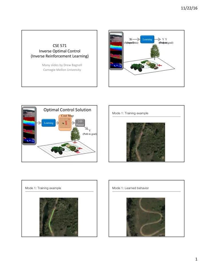
Optimal Control Solution

Learning Y (Path to goal) 2-D Planner

Cost Map Mode 1: Training example Mode 1: Training example Mode 1: Learned behavior

11/22/16 2

Mode 1: Learned behavior Mode 1: Learned cost map Mode 2: Training example Mode 2: Training example Mode 2: Learned behavior Mode 2: Learned behavior

11/22/16 3

Mode 2: Learned cost map Ratliff, Bagnell, Zinkevich 2005 Ratliff, Bradley, Bagnell, Chestnutt, NIPS 2006 Silver, Bagnell, Stentz, RSS 2008 w'

Weighting vector

Cost =

Feature vector

F

w=[], F=[]

Ratliff, Bagnell, Zinkevich, ICML 2006 Ratliff, Bradley, Bagnell, Chestnutt, NIPS 2006 Silver, Bagnell, Stentz, RSS 2008

Learn F1

( , High Cost) ( , Low Cost) w=[w1], F=[F1]

Ratliff, Bagnell, Zinkevich, ICML 2006 Ratliff, Bradley, Bagnell, Chestnutt, NIPS 2006 Silver, Bagnell, Stentz, RSS 2008

Learn F2

( , High Cost) ( , Low Cost)

Ratliff, Bradley, Chesnutt, Bagnell 06 Zucker, Ratliff, Stolle, Chesnutt, Bagnell, Atkeson, Kuffner 09

11/22/16 4

Learned Cost Function Examples Learned Cost Function Examples Learned Cost Function Examples Learning Manipulation Preferences

• Input: Human demonstrations of preferred behavior

(e.g., moving a cup of water upright without spilling)

• Output: Learned cost function that results in trajectories

satisfying user preferences

22 23

Demonstration(s)

24

Demonstration(s) Graph

11/22/16 5

25

Demonstration(s) Graph

26

Demonstration(s) Graph Projection

27

Demonstration(s) Graph Projection

28

Demonstration(s) Graph Projection Learned cost

29

Demonstration(s) Graph Projection Discrete sampled paths Learned cost

30

Demonstration(s) Graph Projection Output trajectories Discrete sampled paths Learned cost

11/22/16 6

31

Demonstration(s) Graph Projection Output trajectories Discrete sampled paths Learned cost Discrete MaxEnt IOC

32

Demonstration(s) Graph Projection Output trajectories Discrete sampled paths Learned cost Local Trajectory Optimization

2D obstacle avoidance task

33

2D state: (x,y)

Graph generation

• Goal: Construct a graph in the robot’s configuration

space providing good coverage

34

Projection

• Goal: Project the continuous demonstration onto the

graph, resulting in a discrete graph path

• Use a modified Dijkstra’s algorithm minimizing sum of:

– Length of discrete path (Euclidean) – Distance to continuous demonstration

35

Learning the cost function

• Goal: Given projected demonstrations, learn the cost

function

• Learn feature weights ( *) using softened value

iteration on the discrete graph (MaxEnt IOC - Ziebart et al., 2008)

– State dependent features (eg: Distance to obstacles)

θ

36

11/22/16 7

Experimental Results

37

Setup

• Binary state-dependent features (~95)
• Histograms of distances to objects
• Histograms of end-effector orientation
• Object specific features (electronic vs non-electronic)
• Approach direction w.r.t goal
• Comparison:
• Human demonstrations
• Obstacle avoidance planner (CHOMP)
• Locally optimal IOC approach (similar to Max-Margin

planning, Ratliff et. al., 2007)

38

Laptop task: Demonstration

( Not part of training set)

39

Laptop task: LTO + Discrete graph path

40

Laptop task: LTO + Smooth random path

41

Statistics for Laptop task

42