
Online Learning Mechanisms for Bayesian Models
- f Word Segmentation
Sharon Goldwater Lisa Pearl Mark Steyvers School of Informatics Department of Cognitive Sciences University of Edinburgh University of California, Irvine Workshop on Psychocomputational Models of Human Language Acquisition VU University Amsterdam, 29 July 2009
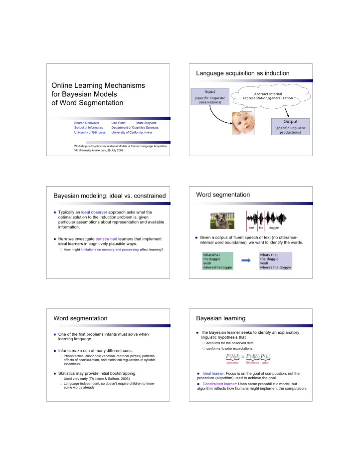
Language acquisition as induction
Input
(specific linguistic
- bservations)
Abstract internal representation/generalization
Output
(specific linguistic productions)
Bayesian modeling: ideal vs. constrained
Typically an ideal observer approach asks what the
- ptimal solution to the induction problem is, given
particular assumptions about representation and available information.
Here we investigate constrained learners that implement
ideal learners in cognitively plausible ways.
How might limitations on memory and processing affect learning?
Word segmentation
Given a corpus of fluent speech or text (no utterance-
internal word boundaries), we want to identify the words.
whatsthat thedoggie yeah wheresthedoggie whats that the doggie yeah wheres the doggie see the doggie
Word segmentation
One of the first problems infants must solve when
learning language.
Infants make use of many different cues. Phonotactics, allophonic variation, metrical (stress) patterns, effects of coarticulation, and statistical regularities in syllable sequences. Statistics may provide initial bootstrapping. Used very early (Thiessen & Saffran, 2003) Language-independent, so doesn’t require children to know some words already
Bayesian learning
The Bayesian learner seeks to identify an explanatory
linguistic hypothesis that
accounts for the observed data. conforms to prior expectations. Ideal learner: Focus is on the goal of computation, not the
procedure (algorithm) used to achieve the goal.
Constrained learner: Uses same probabilistic model, but