On Gradient Descent and Local vs. Global Optimum We conjecture that - PowerPoint PPT Presentation

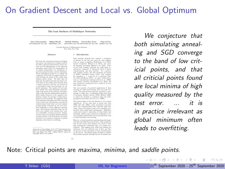
On Gradient Descent and Local vs. Global Optimum We conjecture that both simulating anneal- ing and SGD converge to the band of low crit- icial points, and that all criticial points found are local minima of high quality measured by the test error. ... it is in practice irrelevant as global minimum often leads to overfitting. Note: Critical points are maxima , minima , and saddle points . 21 th September 2020 - 25 th September 2020 T.Stibor (GSI) ML for Beginners

Activation functions Discrimination functions of the form y ( x ) = w T x + w 0 are simple linear functions of the input variables x , where distances are measured by means of the dot product. Let us consider the non-linear logistic sigmoid activation function g ( · ) for limiting the output to (0 , 1), that is, 1 y ( x ) = g ( w T x + w 0 ) , 0.8 0.6 where 0.4 0.2 1 g ( a ) = 0 1 + exp( − a ) -4 -2 0 2 4 a Single-layer network with a logistic sigmoid activation function can also output probabilities (rather than geometric distances). 21 th September 2020 - 25 th September 2020 T.Stibor (GSI) ML for Beginners

Activation functions (cont.) Heaviside step function: 1 0.8 � 0 if a < 0 0.6 g ( a ) = 1 if a ≥ 0 0.4 0.2 0 -4 -2 0 2 4 a Hyperbolic tangent function: 1 g ( a ) = tanh( a ) = exp( a ) − exp( − a ) 0.5 exp( a ) + exp( − a ) 0 Note, tanh( a ) ∈ ( − 1 , 1) -0.5 -1 -4 -2 0 2 4 a 21 th September 2020 - 25 th September 2020 T.Stibor (GSI) ML for Beginners

Activation functions (cont.) Rectified Linear Unit (ReLU) function: g ( a ) = max(0 , a ) Leaky ReLU g ( a ) = max(0 . 1 · a , a ) 21 th September 2020 - 25 th September 2020 T.Stibor (GSI) ML for Beginners

Online/Mini-Batch/Batch Learning Online learning: Update weight w ( i +1) = w ( i ) − η ∂ E ( i ) ∂ w (pattern by pattern). This type of online learning is also called stochastic gradient descent , it is an approximation of the true gradient. Mini-Batch Learning: Partition X randomly in subsets B 1 , B 2 , . . . , B S and � S Update weight w ( i +1) = w ( i ) − η 1 ∂ E ( s ) by computing |B s | s ∂ w derivatives for each pattern in subset B s separately and then sum over all patterns in B s . Batch learning: � N Update weight w ( i +1) = w ( i ) − η 1 ∂ E ( n ) by computing N n =1 ∂ w derivatives for each pattern separately and then sum over all patterns. 21 th September 2020 - 25 th September 2020 T.Stibor (GSI) ML for Beginners

Learning in Neural Networks with Backpropagation minimize 1 2 � f ( W (3) f ( W (2) f ( W (1) X + b (1) ) + b (2) ) + b (3) ) − Y � 2 y 1 y 2 parameters to fit W (3) , b (3) a (2) a (2) a (2) N 2 1 2 W (2) , b (2) a (1) a (1) a (1) 1 2 N 1 W (1) , b (1) x 1 x 2 x D Core idea: Calculate error of loss function and change weights and biases based on output. These “error” measurements for each unit can be used to calculate the partial derivatives. Use partial derivatives with gradient descent for updating weights and biases and minimizing loss function. Problem: At which magnitude one shall change e.g. weight W (1) based on error of y 2 ? ij 21 th September 2020 - 25 th September 2020 T.Stibor (GSI) ML for Beginners

Learning in Neural Networks with Backpropagation (cont.) Input: x 1 , x 2 , output: a (3) 1 , a (3) 2 , target: y 1 , y 2 and g ( · ) is activation function. NN calculates 2 g ( W (2) g ( W (1) x )). � − y 2 ) 2 � ( a (3) − y 1 ) 2 + ( a (3) 2 � a (3) − y � 2 E ( W ) = 1 = 1 2 1 2 a (3) a (3) L 3 1 2 z (3) = W (2) 10 a (2) + W (2) 11 a (2) + W (2) 12 a (2) + W (2) 13 a (2) a (3) = g ( z (2) ) z (3) z (3) 1 0 1 2 3 1 1 1 2 z (3) = W (2) 20 a (2) + W (2) 21 a (2) + W (2) 22 a (2) + W (2) 23 a (2) a (3) = g ( z (2) ) 2 0 1 2 3 2 2 W (2) a (3) = g ( z (3) ) z (3) = W (2) a (2) Forward pass ���� � �� � ���� 2 × 1 2 × 4 4 × 1 a (2) a (2) a (2) L 2 1 2 3 z (2) = W (1) 10 x 0 + W (1) 11 x 1 + W (1) a (2) = g ( z (2) 12 x 2 ) z (2) z (2) z (2) 1 1 1 1 2 3 z (2) = W (1) 20 x 0 + W (1) 21 x 1 + W (1) a (2) = g ( z (2) 22 x 2 ) 2 2 2 z (2) = W (1) 30 x 0 + W (1) 31 x 1 + W (1) a (2) = g ( z (2) 32 x 2 ) 3 3 3 W (1) a (2) = g ( z (2) ) z (2) = W (1) x a (1) a (1) ���� � �� � ���� L 1 1 2 3 × 1 3 × 3 3 × 1 x 1 x 2 2 Notation adapted from Andew Ng’s slides. 21 th September 2020 - 25 th September 2020 T.Stibor (GSI) ML for Beginners

Learning in Neural Networks with Backpropagation (cont.) For each node we calculate δ ( l ) j , that is, error of unit j in layer l , because E ( W ) = a ( l ) j δ ( l +1) ∂ . Note ⊙ is element wise multiplication. i ∂ W ( l ) ij � − y 2 ) 2 � − y 1 ) 2 + ( a (3) 2 � a (3) − y � 2 ( a (3) E ( W ) = 1 = 1 2 1 2 δ (3) = ( a (3) − y ) ⊙ g ′ ( z (3) ) a (3) a (3) L 3 1 2 z (3) z (3) 1 2 W (2) δ (2) = ( W (2) ) T δ (3) ⊙ g ′ ( z (2) ) Backward pass Note δ (1) is the input, so no term. a (2) a (2) a (2) 1 2 3 L 2 z (2) z (2) z (2) 1 2 3 W (1) a (1) a (1) L 1 1 2 x 1 x 2 21 th September 2020 - 25 th September 2020 T.Stibor (GSI) ML for Beginners

Learning in Neural Networks with Backpropagation (cont.) Backpropagation = forward pass & backward pass Given labeled training data ( x 1 , y 1 ) , . . . , ( x N , y N ). Set ∆ ( l ) ij = 0 for all l , i , j . Value ∆ will be used as accumulators for computing partial derivatives. For n = 1 to N Forward pass, compute z (2) , a (2) , z (3) , a (3) , . . . , z ( L ) , a ( L ) Backward pass, compute δ ( L ) , δ ( L − 1) , . . . , δ (2) Accumulate partial derivate terms, ∆ ( l ) := ∆ ( l ) + δ ( l +1) ( a ( l ) ) T Finally calculated partial derivatives for each parameter: N ∆ ( l ) E ( W ) = 1 ∂ and use these in gradient descent. ij ∂ W ( l ) ij See interactive demo. 21 th September 2020 - 25 th September 2020 T.Stibor (GSI) ML for Beginners

Bayes Decision Region vs. Neural Network 2.5 2.0 1.5 y 1.0 0.5 0.0 0 2 4 6 8 10 x Points from blue and red class are generated by a mixture of Gaussians. Black curve shows optimal separation in a Bayes sense. Gray curve shows neural network separation of two independent backpropagation learning runs. 21 th September 2020 - 25 th September 2020 T.Stibor (GSI) ML for Beginners

Neural Network (Density) Decision Region 21 th September 2020 - 25 th September 2020 T.Stibor (GSI) ML for Beginners

Overfitting/Underfitting & Generalization Consider the problem of polynomial curve fitting where we shall fit the data using a polynomial function of the form: M � y ( x , w ) = w 0 + w 1 x + w 2 x 2 + . . . + w M x M = w j x j . j =0 We measure the misfit of our predictive function y ( x , w ) by means of error function which we like to minimize: N � E ( w ) = 1 ( y ( x i , w ) − t i ) 2 2 i =1 where t i is the corresponding target value in the given training data set. 21 th September 2020 - 25 th September 2020 T.Stibor (GSI) ML for Beginners

Polynomial Curve Fitting 1 M = 0 1 M = 1 t t 0 0 −1 −1 0 1 0 1 x x 1 M = 3 1 M = 9 t t 0 0 −1 −1 0 1 0 1 x x 21 th September 2020 - 25 th September 2020 T.Stibor (GSI) ML for Beginners

Polynomial Curve Fitting (cont.) M = 0 M = 1 M = 3 M = 9 0 . 19 0 . 82 0 . 31 0 . 35 w ⋆ 0 w ⋆ − 1 . 27 7 . 99 232 . 37 1 w ⋆ − 25 . 43 − 5321 . 83 2 w ⋆ 17 . 37 48568 . 31 3 w ⋆ − 231639 . 30 4 w ⋆ 640042 . 26 5 w ⋆ − 1061800 . 52 6 w ⋆ 1042400 . 18 7 w ⋆ − 557682 . 99 8 125201 . 43 w ⋆ 9 Table: Coefficients w ⋆ obtained from polynomials of various order. Observe the dramatically increase as the order of the polynomial increases (this table is taken from Bishop’s book). 21 th September 2020 - 25 th September 2020 T.Stibor (GSI) ML for Beginners

Polynomial Curve Fitting (cont.) Observe: if M is too small then the model underfits the data if M is too large then the model overfits the data If M is too large then the model is more flexible and is becoming increasingly tuned to random noise on the target values. It is interesting to note that the overfitting problem become less severe as the size of the data set increases. N = 15 N = 100 1 1 t t 0 0 −1 −1 0 1 0 1 x x ImageNet Classification with Deep ConvolutionalNeural Networks: “The easiest and most common method to reduce overfitting on image data is to artificially enlargethe dataset using label-preserving transformation.” 21 th September 2020 - 25 th September 2020 T.Stibor (GSI) ML for Beginners

Polynomial Curve Fitting (cont.) One technique that can be used to control the overfitting phenomenon is the regularization . Regularization involves adding a penalty term to the error function in order to discourage the coefficients from reaching large values. The modified error function has the form: N � E ( w ) = 1 ( y ( x i , w ) − t i ) 2 + λ � 2 w T w . 2 i =1 By means of the penalty term one reduces the value of the coefficients (shrinkage method). 21 th September 2020 - 25 th September 2020 T.Stibor (GSI) ML for Beginners

Regularized Polynomial Curve Fitting M = 9 ln λ = − 18 1 t 0 −1 0 1 x 21 th September 2020 - 25 th September 2020 T.Stibor (GSI) ML for Beginners