numerical integration for local positioning
play

Numerical Integration for Local Positioning Niilo Sirola, Robert - PowerPoint PPT Presentation

Numerical Integration for Local Positioning Niilo Sirola, Robert Pich e, Henri Pesonen Tampere University of Technology, Tampere, Finland x p ( r | x ) d x x = p ( r | x ) d x Sirola, Pich e, Pesonen: Numerical


  1. Numerical Integration for Local Positioning Niilo Sirola, Robert Pich´ e, Henri Pesonen Tampere University of Technology, Tampere, Finland
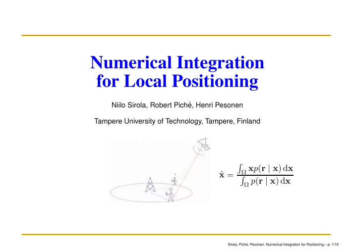
 � Ω x p ( r | x ) d x x = ˆ � Ω p ( r | x ) d x Sirola, Pich´ e, Pesonen: Numerical Integration for Positioning – p. 1/15

  2. Nokia funds positioning & tracking research at TUT/math Since 2000 we’ve studied and developed Algorithms to compute satellite orbits GPS position without nav. data Exact solutions for hybrid GPS/cellular positioning Tracking filters (Kalman, Particle Monte Carlo) See alpha.cc.tut.fi/ ∼ niilo/posgroup/ Sirola, Pich´ e, Pesonen: Numerical Integration for Positioning – p. 2/15

  3. Local positioning presents special problems When reference stations are nearby, geometry is strongly nonlinear and measurement errors are nongaussian. EKF may choose the wrong track and underestimate error: Sirola, Pich´ e, Pesonen: Numerical Integration for Positioning – p. 3/15

  4. Bayes’ formula provides a basis for estimation A measurement r is a realisation of a r.v. with pdf p ( r | x ) . Prior knowledge is modelled by pdf p ( x ) . The posterior pdf is p ( r | x ) p ( x ) p ( x | r ) = � p ( r | x ) p ( x ) d x An estimate is the mean of the posterior: � x = ˆ x p ( x | r ) d x x � 2 p ( x | r ) d x d r �� This minimizes � x − ˆ Sirola, Pich´ e, Pesonen: Numerical Integration for Positioning – p. 4/15

  5. Position estimation from range measurements If r i = � s i − x � + ǫ i with ǫ i ∼ φ i then p ( r i | x ) = φ i ( � s i − x � − r i ) If measurements are independent then � p ( r | x ) = φ i ( � s i − x � − r i ) i Assume prior pdf p ( x ) = constant in cell Ω The Bayesian position estimate is � Ω x p ( r | x ) d x x = ˆ � Ω p ( r | x ) d x Sirola, Pich´ e, Pesonen: Numerical Integration for Positioning – p. 5/15

  6. Bayesian position estimation example p ( r 1 | x ) p ( x ) Sirola, Pich´ e, Pesonen: Numerical Integration for Positioning – p. 6/15

  7. Another bayesian position estimation example p ( r 2 | x ) p ( x ) Sirola, Pich´ e, Pesonen: Numerical Integration for Positioning – p. 7/15

  8. Now combine the previous two examples p ( r | x ) p ( x ) Sirola, Pich´ e, Pesonen: Numerical Integration for Positioning – p. 8/15

  9. Many multidimensional quadrature methods are available Ω f ( x ) d x as | Ω | � N Monte Carlo estimates � i =1 f ( x i ) , where x i N are uniformly distributed random samples. quasi-Monte Carlo uses a deterministic sequence of samples. grid method uses values on a uniform regular grid. subregion adaptive quadrature locally refines the grid and the degrees of piecewise polynomials (C UBPACK ). Monte Carlo Adaptive cubature Grid Quasi Monte Carlo Sirola, Pich´ e, Pesonen: Numerical Integration for Positioning – p. 9/15

  10. Compare quadrature methods using test cases We generated several posterior pdfs of the form 2 � � ( � s i − x � − r i ) 2 − 1 � p ( x | r ) ∝ exp σ 2 2 i i =1 over 1 km × 1 km with 50m ≤ σ i ≤ 150m. unimodal bimodal Sirola, Pich´ e, Pesonen: Numerical Integration for Positioning – p. 10/15

  11. All three methods can estimate their accuracy Error / m 10 2 10 Quasi-Monte Carlo 1 Cubpack 10-1 Grid -2 10 0 1000 2000 3000 4000 5000 No of samples Sirola, Pich´ e, Pesonen: Numerical Integration for Positioning – p. 11/15

  12. Grid and C UBPACK usually beat Monte Carlo How frequently (%) each method gave the best answer. 500 samples unimodal bimodal C UBPACK 41 77 Grid 73 24 Quasi Monte Carlo 3 4 5000 samples 10000 samples C UBPACK 100 98 C UBPACK 100 98 Grid 83 16 Grid 93 28 Quasi-MC 36 31 Quasi-MC 54 50 Sirola, Pich´ e, Pesonen: Numerical Integration for Positioning – p. 12/15

  13. Grid and C UBPACK beat Monte Carlo overall 600 test cases, each with 500 samples: Bimodal Unimodal 0.95 0.95 0.90 0.90 Grid Cubpack 0.50 0.50 probability Cubpack Grid Quasi-MC 0.10 0.10 0.01 0.01 Quasi-MC 0.01 0.1 1 10 100 1000 0.01 0.1 1 10 100 1000 Error / m Error / m 10000 samples Bimodal Unimodal Cubpack Cubpack 0.95 0.95 Grid Grid 0.90 0.90 Quasi-MC Quasi-MC 0.50 0.50 0.10 0.10 0.01 0.01 0.01 0.1 1 10 100 1000 0.01 0.1 1 10 100 1000 Error / m Error / m Sirola, Pich´ e, Pesonen: Numerical Integration for Positioning – p. 13/15

  14. The Monte Carlo method improves in 3D 100 test cases, each with 1000 samples bimodal unimodal 0.95 0.95 0.90 0.90 0.50 0.50 Cubpack Cubpack Quasi-MC Quasi-MC 0.10 0.10 Grid Grid 0.01 0.01 0.01 0.1 1 10 100 1000 0.01 0.1 1 10 100 1000 How frequently (%) each method gave the best answer: unimodal bimodal C UBPACK 73 75 Grid 7 1 Quasi-MC 69 74 Sirola, Pich´ e, Pesonen: Numerical Integration for Positioning – p. 14/15

  15. Conclusions, Further Directions To compute 2D and 3D integrals in Bayesian positioning, subregion-adaptive quadrature outperforms plain Monte-Carlo methods, especially for quadrature error estimation and (overly?) high precision. Both approaches can be improved by exploiting special features of the problem. Both approaches can be used in Bayesian tracking. � Ω x p ( r | x ) d x x = ˆ � Ω p ( r | x ) d x Sirola, Pich´ e, Pesonen: Numerical Integration for Positioning – p. 15/15

Download Presentation
Download Policy: The content available on the website is offered to you 'AS IS' for your personal information and use only. It cannot be commercialized, licensed, or distributed on other websites without prior consent from the author. To download a presentation, simply click this link. If you encounter any difficulties during the download process, it's possible that the publisher has removed the file from their server.

Recommend


More recommend