
SLIDE 1
NP Completeness
- Tractability
- Polynomial time
- Computation vs. verification
- Power of non-determinism
- Encodings
- Transformations & reducibilities
- P vs. NP
- “Completeness”
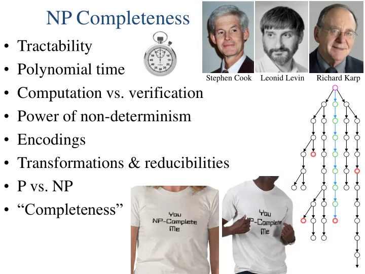
Stephen Cook Leonid Levin Richard Karp