Notes Trapezoidal Rule Again Most of assignment 1 hasn t been - - PowerPoint PPT Presentation

1 cs533d-term1-2005

Notes

Most of assignment 1 hasnt been covered

in class yet, but after today you should be able to do a lot of it

Forgot to include instructions about

view_obj:

• To navigate, hold down shift and click/drag

with left, right, or middle mouse buttons (same navigation model as Maya)

2 cs533d-term1-2005

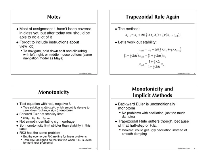
Trapezoidal Rule Again

The method: Lets work out stability:

xn+1 = xn + t

1 2 v(xn,tn) + 1 2 v(xn+1,tn+1)

( )

xn+1 = xn + t

1 2 xn + 1 2 xn+1

( )

1 1

2 t

( )xn+1 = 1+ 1

2 t

( )xn

xn+1 = 1+ 1

2

1 1

2 t xn

3 cs533d-term1-2005

Monotonicity

Test equation with real, negative

• True solution is x(t)=x0et, which smoothly decays to

zero, doesnt change sign (monotone)

Forward Euler at stability limit:

• x=x0, -x0, x0, -x0, …

Not smooth, oscillating sign: garbage! So monotonicity limit stricter than stability in this

case

RK3 has the same problem

• But the even order RK are fine for linear problems
• TVD-RK3 designed so that its fine when F.E. is, even

for nonlinear problems!

4 cs533d-term1-2005

Monotonicity and Implicit Methods

Backward Euler is unconditionally

monotone

• No problems with oscillation, just too much

damping

Trapezoidal Rule suffers though, because

• f that half-step of F.E.
• Beware: could get ugly oscillation instead of

smooth damping

5 cs533d-term1-2005

Summary 1

Particle Systems: useful for lots of stuff Need to move particles in velocity field Forward Euler

• Simple, first choice unless problem has
• scillation/rotation

Runge-Kutta if happy to obey stability limit

• Modified Euler may be cheapest method
• RK4 general purpose workhorse
• TVD-RK3 for more robustness with

nonlinearity (more on this later in the course!)

6 cs533d-term1-2005

Summary 2

If stability limit is a problem, look at implicit

methods

• e.g. need to guarantee a frame-rate, or

explicit time steps are way too small

Trapezoidal Rule

• If monotonicity isnt a problem

Backward Euler

• Almost always works, but may over-damp!

7 cs533d-term1-2005

Second Order Motion

8 cs533d-term1-2005

Second Order Motion

If particle state is just position (and colour, size, …) then

1st order motion

• No inertia
• Good for very light particles that stay suspended: smoke, dust…
• Good for some special cases (hacks)

But most often, want inertia

• State includes velocity, specify acceleration
• Can then do parabolic arcs due to gravity, etc.

This puts us in the realm of standard Newtonian physics

• F=ma

Alternatively put:

• dx/dt=v
• dv/dt=F(x,v,t)/m (i.e. a(x,v,t) )

For systems (with many masses) say dv/dt=M-1F(x,v,t)

where M is the “mass matrix” - masses on the diagonal

9 cs533d-term1-2005

What’s New?

If x=(x,v) this is just a special form of 1st

• rder: dx/dt=v(x,t)

But since we know the special structure,

can we take advantage of it? (i.e. better time integration algorithms)

• More stability for less cost?
• Handle position and velocity differently to

better control error?

10 cs533d-term1-2005

Linear Analysis

Approximate acceleration: Split up analysis into different cases Begin with first term dominating:

constant acceleration

• e.g. gravity is most important

a x,v

( ) a0 + a

x x + a v v

11 cs533d-term1-2005

Constant Acceleration

Solution is No problem to get v(t) right:

just need 1st order accuracy

But x(t) demands 2nd order accuracy So we can look at mixed methods:

• 1st order in v
• 2nd order in x

v(t) = v0 + a0t x(t) = x0 + v0t + 1

2 a0t 2

12 cs533d-term1-2005

Dependence on x and v dominates:

a(x,v)=-Kx-Dv

Do the analysis as before: Eigenvalues of this matrix?

d dt x v

• =

I K D

• x

v

• Linear Acceleration

13 cs533d-term1-2005

More Approximations…

Typically K and D are symmetric semi-definite

(there are good reasons)

• What does this mean about their eigenvalues?

Often, D is a linear combination of K and I

(“Rayleigh damping”), or at least close to it

• Then K and D have the same eigenvectors

(but different eigenvalues)

• Then the eigenvectors of the Jacobian are of the form

(u, u)T

• [work out what is in terms of K and D]

14 cs533d-term1-2005

Simplification

is the eigenvalue of the Jacobian, and Same as eigenvalues of Can replace K and D (matrices) with

corresponding eigenvalues (scalars)

• Just have to analyze 2x2 system

= 1

2 D ± 1 2 D

( )

2 K

1 K D

• 15

cs533d-term1-2005

Split Into More Cases

Still messy! Simplify further If D dominates (e.g. air drag, damping)

• Exponential decay and constant

If K dominates (e.g. spring force)

D, 0

{ }

± 1 K

16 cs533d-term1-2005

Three Test Equations

Constant acceleration (e.g. gravity)

• a(x,v,t)=g
• Want exact (2nd order accurate) position

Position dependence (e.g. spring force)

• a(x,v,t)=-Kx
• Want stability but low or zero damping
• Look at imaginary axis

Velocity dependence (e.g. damping)

• a(x,v,t)=-Dv
• Want stability, monotone decay
• Look at negative real axis

17 cs533d-term1-2005

Explicit methods from before

Forward Euler

• Constant acceleration: bad (1st order)
• Position dependence: very bad (unstable)
• Velocity dependence: ok (conditionally

monotone/stable)

RK3 and RK4

• Constant acceleration: great (high order)
• Position dependence: ok (conditionally stable, but

damps out oscillation)

• Velocity dependence: ok (conditionally

monotone/stable)

18 cs533d-term1-2005

Implicit methods from before

Backward Euler

• Constant acceleration: bad (1st order)
• Position dependence: ok (stable, but damps)
• Velocity dependence: great (monotone)

Trapezoidal Rule

• Constant acceleration: great (2nd order)
• Position dependence: great (stable, no

damping)

• Velocity dependence: good (stable but only

conditionally monotone)

19 cs533d-term1-2005

Setting Up Implicit Solves

Lets take a look at actually using Backwards

Euler, for example

Eliminate position, solve for velocity: Linearize at guess vk, solving for vn+1 vk+v Collect terms, multiply by M

xn+1 = xn + t vn+1 vn+1 = vn + t M 1F xn+1,vn+1

( )

vn+1 = vn + t M 1F xn + t vn+1,vn+1

( )

vk + v = vn + t M 1 F xn + tvk,vk

( )+ t F

x v+ F v v

• M t F

v t 2 F x

• v = M vn vk

( )+ t F xn + tvk,vk ( )

20 cs533d-term1-2005

Symmetry

Why multiply by M? Physics often demands that and

are symmetric

• And M is symmetric, so this means matrix is

symmetric, hence easier to solve

• (physics generally says matrix is SPD - even better)
• If the masses are not equal, the acceleration form of

the equations results in an unsymmetric matrix - bad.

Unfortunately the matrix is usually

unsymmetric

• Makes solving with it considerably less efficient
• See Baraff & Witkin, “Large steps in cloth simulation”,

SIGGRAPH 98 for one solution: throw out bad part Fposition x F

velocity

v F

velocity

x

21 cs533d-term1-2005

Specialized 2nd Order Methods

This is again a big subject Again look at explicit methods, implicit

methods

Also can treat position and velocity

dependence differently: mixed implicit-explicit methods

22 cs533d-term1-2005

Symplectic Euler

Like Forward Euler, but updated velocity used

for position

Some people flip the steps (= relabel vn) Symplectic means certain qualities of the

underlying physics are preserved in discretization - quite desirable visually!

[work out test cases]

vn+1 = vn + ta xn,vn

( )

xn+1 = xn + tvn+1

23 cs533d-term1-2005

Constant acceleration: bad

• Velocity right, position off by O(t)

Position dependence: good

• Stability limit
• No damping! (symplectic)

Velocity dependence: ok

• Monotone limit
• Stability limit

t < 2 K

t <1 D t < 2 D

Symplectic Euler performance

24 cs533d-term1-2005

Tweaking Symplectic Euler

[sketch algorithms] Stagger the velocity to improve x Start off with Then proceed with Finish off with

v 12 = v0 + 1

2 ta x0,v0

( )

vn+ 12 = vn 12 + 1

2 (tn+1 tn1)a xn,vn 12

( )

xn+1 = xn + tvn+ 12 vN = vN 12 + 1

2 ta xN,vN 12

( )

25 cs533d-term1-2005

Staggered Symplectic Euler

Constant acceleration: great!

• Position is exact now

Other cases not effected

• Was that magic? Main part of algorithm unchanged

(apart from relabeling) yet now its more accurate!

Only downside to staggering

• At intermediate times, position and velocity not known

together

• May need to think a bit more about collisions and
• ther interactions with outside algorithms…

26 cs533d-term1-2005

A common explicit method

May see this one pop up: Constant acceleration: great Velocity dependence: ok

• Conditionally stable/monotone

Position dependence: BAD

• Unconditionally unstable!

vn+1 = vn + ta xn,vn

( )

xn+1 = xn + t

1 2 vn + 1 2 vn+1

( ) = xn + tvn + 1

2 t 2an

27 cs533d-term1-2005

An Implicit Compromise

Backward Euler is nice due to

unconditional monotonicity

• Although only 1st order accurate, it has the

right characteristics for damping

Trapezoidal Rule is great for everything

except damping with large time steps

• 2nd order accurate, doesnt damp pure
• scillation/rotation

How can we combine the two?

28 cs533d-term1-2005

Implicit Compromise

Use Backward Euler for velocity dependence,

Trapezoidal Rule for the rest:

Constant acceleration: great (2nd order) Position dependence: great (2nd order, no

damping)

Velocity dependence: great (unconditionally

monotone)

xn+1 = xn + t

1 2 vn + 1 2 vn+1

( )

vn+1 = vn + ta 1

2 xn + 1 2 xn+1,vn+1,tn+ 12

( )