Notes on Support Vector Machines, COMP24111 Tingting Mu - - PDF document

SLIDE 1

Notes on Support Vector Machines, COMP24111

Tingting Mu

tingtingmu@manchester.ac.uk School of Computer Science University of Manchester Manchester M13 9PL, UK Editor: NA

We start from introducing the notations to be used in this notes. We denote a set of training samples by {(x1,y1),(x2,y2),...,(xN,yN)}. The column vector xi ∈ Rd denotes the d-dimensional feature vector of the i-th training sample, which corresponds to a data point in a d-dimensional space. The scalar yi ∈ {−1,+1} denotes the class label of the i-th training sample, for which +1 represents the positive class while −1 the negative class1.

• 1. Support Vector Machines

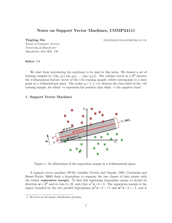
x1 x2

2 / | | w | |2

w wTx+b=0 wTx+b=-1 w

T

x+b=1 ρ ρ

Figure 1: An illustration of the separation margin in a 2-dimensional space. A support vector machine (SVM) classifier (Cortes and Vapnik, 1995; Cristianini and Shawe-Taylor, 2000) finds a hyperplane to separate the two classes of data points with the widest separation margin. To find this separating hyperplane means to decide its direction w ∈ Rd and its bias b ∈ R, such that wT x + b = 0. The separation margin is the region bounded by the two parallel hyperplanes wT x + b = +1 and wT x + b = −1, and is

• 1. We focus on the binary classification problem.

1

SLIDE 2

computed by: margin = 2ρ = 2 ∥w∥2 = 2 √ wT w . (1) Figure 1 illustrates a separating hyperplane, as well as the two parallel hyperplanes associ- ated with it, and its separation margin. In addition to margin maximisation, the SVM classifier attempts to prevent the two classes of data points from falling into the margin. To achieve this, it forces wT x + b ≥ 1 for a sample (x,+1) from the positive class, while wT x + b ≤ 1 for a sample (x,−1) from the negative class. This is equivalent to forcing y (wT x + b) ≥ 1 for any given sample (x,y) where y ∈ {−1,+1}. 1.1 Hard Margin SVM To maximise the separation margin in Eq. (1) is equivalent to minimising the term wT w. To enforce all the training samples stay outside the margin is equivalent to setting the constraints of yi (wT xi + b) ≥ 1 for i = 1,2,...,N. Together, this gives the following con- strained optimisation problem to solve: min

w∈Rd,b∈R

1 2wT w, (2) subject to yi (wT xi + b) ≥ 1, for i = 1,2,...,N. (3)

• Eq. (2) is referred to as the objective function of the optimisation problem. The purpose
• f introducing the scaling factor 1

2 in Eq. (2) is to have a neat gradient form (w instead

• f 2w). The SVM training refers to the process of finding the optimal values of w and b.

The solution gives us the hard margin SVM classifier, which is also called the optimal margin classifier. 1.2 1-Norm Soft Margin SVM When processing real-world data, we often need to deal with non-separable data patterns (see Figure 2 for example), for which it is impossible to find a hyperplane to separate perfectly the two classes. In this situation, it is helpful to allow the margin constraints in

• Eq. (3) to be violated.

We use the slack variable ξi ≥ 0 to measure the deviation from the ideal situation yi (wT xi + b) ≥ 1 for the i-th training sample. A set of more relaxed constraints are used instead: yi (wT xi + b) ≥ 1 − ξi, for i = 1,2,...,N. (4) When 0 < ξi < 1, the corresponding sample point is allowed to fall within the margin region, but still has to be in the right side. When ξi = 1, the corresponding point is allowed to stay

• n the decision boundary. When ξi > 1, the point is allowed to stay in the wrong side of the

decision boundary. Although we relax the constraints to allow Eq. (3) to be violated, the violation, which is measured by the strength of ξi (e.g., ∣ξi∣), should be small to maintain good accuracy. For instance, it is not wise to build a classifier that allows most training samples to fall in the wrong side of the separating hyperplane. Therefore, we minimise the term ∑N

i=1 ∣ξi∣, which is

2

SLIDE 3

equal to ∑N

i=1 ξi since all the slack variables are positive numbers, together with the margin

term 1

2wT w. The modified constrained optimisation problem becomes

min

w∈Rd,b∈R

1 2wT w + C

N

∑

i=1

ξi, (5) subject to yi (wT xi + b) ≥ 1 − ξi, for i = 1,2,...,N, (6) ξi ≥ 0, for i = 1,2,...,N, (7) where C > 0 is called the regularisation parameter. Let the column vector ξ = [ξ1,ξ2,...ξN]T store the slack variables and we refer to it as a slack vector. The second term in the

• bjective function in Eq. (5) can be expressed via l1-norm C∥ξ∥1. This modified SVM is

subsequently named as the 1-norm soft margin SVM, and is often referred to as the l1-SVM for simplification.

x1 x2

Figure 2: Illustration of an case of non-separable data patterns. 1.3 Support Vectors The training samples that (1) distribute along one of the two parallel hyperplanes, or (2) fall within the margin, or (3) stay in the wrong side of the separating hyperplane are more challenging to classify. They contribute more significantly to the determination of the direction and position of the separating hyperplane. They are called support vectors. The other samples that are not only stay in the right side of the separating hyperplane but also stay outside the margin are called non-support vectors, and they affect less the position

• f the separating hyperplane.
• 2. Dual Problem of SVM (Optional Reading)

An SVM classifier can be trained by solving a quadratic programming (QP) problem. This QP problem is called the dual problem of an SVM. A QP problem is a special type

• f optimisation problem, and there exist many sophisticated approaches for solving it. Its

3

SLIDE 4

• bjective function is a quadratic function of multiple input variables and its constraint

functions are linear functions of these variables. We will explain in this section how to derive this dual problem by using the method of Lagrange multipliers. 2.1 Lagrange Duality We start from introducing some knowledge on how to solve a constrained optimisation problem using the method of Lagrange multipliers. A general way to describe a constrained

• ptimisation problem is

min

x∈Rn

f(x), (8) subject to gi(x) ≤ 0, for i = 1,2,...,K, (9) hi(x) = 0, for i = 1,2,...,L. (10) The above expression means that we would like to find the optimal value of the vector x so that the value of the function f(x) ∶ Rn → R is minimised, meanwhile the optimal x has to satisfy a total of K different inequality constraints {gi(x) ≤ 0}K

i=1 and a total of L different

equality constraints {hi(x) = 0}L

i=1. Here, gi(x) ∶ Rn → R and hi(x) ∶ Rn → R are constraint

functions, which take the same input variables as f(x). An effective way for solving the constrained optimisation problem in Eqs. (8)-(10) is the method of Lagrange multipliers. It first constructs a Lagrangian function by adding the constraint functions to the objective function, resulting in L(x,{λi}K

i=1,{βi}L i=1) = f(x) + K

∑

i=1

λigi(x) +

L

∑

i=1

βihi(x), (11) where we call {λi}K

i=1 and {βi}L i=1 Lagrange multipliers. Storing the Lagrange multipli-

ers in two column vectors such that λ = [λ1,λ2,...,λK]T and β = [β1,β2,...,βL]T , the Lagrangian function is denoted by L(x,λ,β). The original constrained optimisation problem in Eqs. (8)-(10) is called the primal

• problem. To assist solving it, a dual problem is imposed using the above Lagrangian
• function. It is given as

max

λ∈RK,β∈RL

O(λ,β), (12) subject to λi ≥ 0, for i = 1,2,...,K, (13) where O(λ,β) = min

x∈Rn L(x,λ,β).

(14) Under certain assumptions2 on the objective and constraint functions f, {gi}K

i=1 and

{hi}L

i=1, there must exist a setting of x and λ and β, denoted by x∗ and λ∗ and β∗, so

that x∗ is the optimal solution of the primal problem in Eqs. (8)-(10), and {λ∗,β∗} is the

• 2. We do not discuss details on the assumptions. It is proven that the objective and constraint functions
• f the SVM problems satisfy these assumptions.

4

SLIDE 5

• ptimal solution of the dual problem in Eqs. (12)- Eq. (13), also x∗ is the optimal solution
• f Eq. (14). This means x∗ and λ∗ and β∗ need to satisfy the following optimal conditions:

∂ ∂xi L(x∗,λ∗,β∗) = 0, for i = 1,2,...,N, (stationarity), (15) hi(x∗) = 0, for i = 1,2,...,L, (primal feasibility), (16) gi(x∗) ≤ 0, for i = 1,2,...,K, (primal feasibility), (17) λ∗

i ≥ 0, for i = 1,2,...,K,

(dual feasibility), (18) λ∗

i gi(x∗) = 0, for i = 1,2,...,K,

(complementary slackness). (19) These conditions are called the Karush-Kuhn-Tucker (KKT) conditions, where Eq. (15) is known as the stationarity condition, Eqs. (16) and (17) the primal feasibility, Eq. (18) the dual feasibility, and Eq. (19) the complementary slackness. If you can find some x, λ and β that satisfy the KKT conditions, then these must be solutions to the primal and dual problems. To summarise, to solve a constrained optimisation problem using the method of La- grange multipliers, its Lagrangian function is firstly constructed based on Eq. (11). Then, the dual problem is constructed based on Eqs. (12)-(14). During the optimisation, the KKT conditions are examined. 2.2 Dual Problem of Hard Margin SVM 2.2.1 Derive the Dual Problem We derive the dual problem for the hard margin SVM in Eqs. (2)-(3) as a practice. The variables to be optimised for the hard margin SVM are stored in the vector [ w b ], consti- tuting a (d + 1)-dimensional vector. The objective function is 1

2wT w. There are a total of

K = N inequality constraint functions, each formed for a training sample, given as 1 − yi (wT xi + b) ≤ 0. (20) There is no equality constraint in the SVM problem. You could also treat this as setting all the equality constraint functions as zeros: hi(x) = 0. Following Eq. (11), we define the Lagrangian function as L(w,b,{λi}N

i=1) = 1

2wT w +

N

∑

i=1

λi [1 − yi (wT xi + b)]. (21) Next, we show how to construct the dual problem. We first compute the objective function O ({λi}K

i=1) for the dual problem according to Eq. (14). We have learned that the

minimum of a function is reached when its gradient reaches zero. Therefore, to minimise the Lagrangian function with respect to w and b, we first calculate the gradient. The Lagrangian function can be re-written as L(w,b,{λi}N

i=1) = 1

2wT w − wT (

N

∑

i=1

λiyixi) +

N

∑

i=1

λi(1 − byi). (22) 5

SLIDE 6

It includes one quadratic function 1

2wT w, one linear function wT (∑N i=1 λiyixi), and one

constant function of w. Applying the gradient calculation rules for linear and quadratic functions as shown in the maths notes, we have ∂ ∂wL(w,b,{λi}N

i=1) = w − N

∑

i=1

λiyixi. (23) Since the only term in the Lagrangian function that is related to b is −b∑N

i=1 λiyi, we have

∂ ∂bL(w,b,{λi}N

i=1) = − N

∑

i=1

λiyi. (24) Set the gradient to zero so that

∂ ∂wL(w,b,{λi}N i=1) = 0 and ∂ ∂bL(w,b,{λi}N i=1) = 0. This

corresponds to the stationarity condition in Eq. (15), and it results in w =

N

∑

i=1

λiyixi, (25)

N

∑

i=1

λiyi = 0. (26) Replacing w with ∑N

i=1 λiyixi and replacing ∑N i=1 λiyi with zero in the Lagrangian function

in Eq. (21), the optimised Lagrangian function with respect to w is obtained by O ({λi}N

i=1)

= 1 2

N

∑

i=1 N

∑

j=1

λiλjyiyjxT

i xj − N

∑

i=1 N

∑

j=1

λiλjyiyjxT

i xj + N

∑

i=1

λi = −1 2

N

∑

i=1 N

∑

j=1

λiλjyiyjxT

i xj + N

∑

i=1

λi. (27) This is a function of the Lagrange multipliers, which is the objective function of the dual problem of the hard margin SVM. According to the dual feasibility condition in Eq. (18), λi needs to be non-negative. Also Eq. (26) needs to hold. Subsequently, the complete formulation of the dual problem to be solved for the hard-margin SVM is given as max

{λi}N

i=1

−1 2

N

∑

i=1 N

∑

j=1

λiλjyiyjxT

i xj + N

∑

i=1

λi, (28) subject to λi ≥ 0, for i = 1,2,...,N, (29)

N

∑

i=1

λiyi = 0. (30) This is a QP problem and its solution will be discussed later. 2.2.2 From Complementary Slackness Condition to Support Vectors Additionally, the complementary slackness condition λ∗

i [1 − yi (xT i w∗ + b∗)] = 0 needs to be

satisfied for each training sample. This gives the concept of the support vector. After the 6

SLIDE 7

training, the training samples that are assigned non-zero Lagrange multipliers must satisfy 1 − yi (xT

i w∗ + b∗) = 0. These sample points distribute along the two parallel hyperplanes,

and are called support vectors. The remaining training samples with λ∗

i = 0 can have

nonzero values of 1 − yi (xT

i w∗ + b∗), more specifically yi (xT i w∗ + b∗) > 1 according to Eq.

(20). These sample points stay outside the margin and are called non-support vectors. 2.2.3 From Dual Solution to SVM Decision Function The primal feasibility condition in Eq. (17) tells us yi(wT xi +b) ≥ 1. Therefore, among the training samples from the positive class, the one possessing the lowest prediction function value, which is found by I+ = arg min

yi=+1xT i w∗ + b∗,

(31) should be the closest to the upper parallel hyperplane and should satisfy xT

I+w∗ + b∗ = 1,

(32) Similarly, among the training samples from the negative class, the one possessing the highest prediction function value, which is found by I− = arg max

yi=−1xT i w∗ + b∗,

(33) should be the closest to the lower parallel hyperplane and should satisfy xT

I−w∗ + b∗ = −1.

(34) The optimal value of b can then be approximated by adding Eqs. (32) and (34), which gives b∗ = − xT

I+w∗ + xT I−w∗

2 . (35) An equivalent expression of the above b∗ is b∗ = −minyi=+1 xT

i w∗ + maxyi=−1 xT i w∗

2 . (36) Incorporating Eq. (25), the final prediction function of the SVM is computed by ˆ y = xT w∗ + b∗ =

N

∑

i=1

λ∗

i yixT xi − minyi=+1 xT i w∗ + maxyi=−1 xT i w∗

2 =

N

∑

i=1

λ∗

i yixT xi − minyk=+1 ∑N i=1 λ∗ i yixT k xi + maxyk=−1 ∑N i=1 λ∗ i yixT k xi

2 . (37) The above equation shows how the optimal solution {λ∗

i }N i=1 of the QP problem can be used

to build a hard margin SVM classifier. 7

SLIDE 8

2.3 Dual Problem of 1-Norm Soft Margin SVM (l1-SVM) 2.3.1 Derive the Dual Problem In this section, we show how to derive the dual problem for the l1-SVM. The variables to be optimised are stored in the vector ⎡ ⎢ ⎢ ⎢ ⎢ ⎢ ⎣ w ξ b ⎤ ⎥ ⎥ ⎥ ⎥ ⎥ ⎦ , constituting a (d + N + 1)-dimensional vector. The objective function is 1

2wT w + C∣ξ∣1. There are a total of K = 2N inequality constraint

functions, where two inequality constraints are required for each of the N training samples: 1 − ξi − yi (wT xi + b) ≤ 0, (38) −ξi ≤ 0. (39) Similar to the hard margin SVM, there is no equality constraint. We first construct the Lagrangian function by following Eq. (11): L(w,ξ,b,{αi}N

i=1,{βi}N i=1) = 1

2wT w +C∣ξ∣1 +

N

∑

i=1

αi [1 − ξi − yi (wT xi + b)]+

N

∑

i=1

βi(−ξi). (40) Here, a total of 2N Lagrange multipliers {αi,βi ≥ 0}N

i=1 are used since there are a total of

2N inequality constraints. The vectors α = [α1,α2,...,αN]T and β = [β1,β2,...,βN]T are used to store the Lagrange multipliers. Next we construct the dual problem. Because the objective function of the dual problem is obtained by minimising the Lagrangian function with respect to ⎡ ⎢ ⎢ ⎢ ⎢ ⎢ ⎣ w ξ b ⎤ ⎥ ⎥ ⎥ ⎥ ⎥ ⎦ , we need to compute the gradient of the Lagrangian function, which is given by ∂ ∂wL(w,ξ,b,{αi}N

i=1,{βi}N i=1)

= w −

N

∑

i=1

λiyixi, (41) ∂ ∂ξi L(w,ξ,b,{αi}N

i=1,{βi}N i=1)

= C − (αi + βi), for i = 1,2,...,N, (42) ∂ ∂bL(w,ξ,b,{αi}N

i=1,{βi}N i=1)

= −

N

∑

i=1

αiyi. (43) Here, we do not explain the gradient calculation in details, as it follows a similar procedure as in the hard margin SVM. Setting the gradient to zero, we have w =

N

∑

i=1

λiyixi, (44) C = αi + βi, for i = 1,2,...,N, (45)

N

∑

i=1

αiyi = 0. (46) Replacing w with ∑N

i=1 λiyixi, replacing αi + βi with C, and ∑N i=1 αiyi with zero, the formu-

lation of the optimised Lagrangian function with respect to w, ξ and b is obtained: O(α,β) = −1 2

N

∑

i=1 N

∑

j=1

αiαjyiyjxT

i xj + N

∑

i=1

αi. (47) 8

SLIDE 9

• Eq. (45) indicates that the values of αi and βi cannot exceed C, because the Lagrange

multipliers αi and βi are non-negative. This is used as an extra constraint for each Lagrange

• multiplier. The final dual problem of the l1-SVM is given by

max

{αi}N

i=1

−1 2

N

∑

i=1 N

∑

j=1

αiαjyiyjxT

i xj + N

∑

i=1

αi, (48) subject to 0 ≤ αi ≤ C, for i = 1,2,...,N, (49)

N

∑

i=1

αiyi = 0. (50) Comparing the dual problem of the l1-SVM in Eqs. (48)-(50) and the dual problem of the hard margin SVM in Eqs. (28)-(30), it is interesting to see that they actually share the same objective function. The difference is that an extra upper bound C is applied to the Lagrange multipliers of the l1-SVM. The Lagrange multipliers {βi}N

i=1 of the l1-SVM do not

play any role in the optimisation. 2.3.2 From Complementary Slackness Condition to Support Vectors The complementary slackness conditions to be satisfied for each training sample include α∗

i [1 − ξ∗ i − yi (xT i w∗ + b∗)] = 0,

(51) β∗

i ξi = (C − α∗ i )ξi = 0.

(52) We observe the obtained value α∗

i for each training sample.

Figure 3: An illustration of support vectors for linear, non-separable patterns. The figure is from Mu and Nandi (2007). 9

SLIDE 10

When 0 < α∗

i < C, Eq. (52) indicates ξ∗ i = 0 and Eq. (51) indicates 1−ξ∗ i −yi (xT i w∗ + b∗) =

• 0. Combining these two equations, we have 1 − yi (xT

i w∗ + b∗) = 0. Therefore, the train-

ing samples that possess 0 < α∗

i < C distribute along one of the two parallel hyperplanes

(either xT

i w∗ + b∗ = +1 or xT i w∗ + b∗ = −1), which are called margin support vectors.

Those training samples possessing α∗

i = C can have non-zero ξi, which then have to satisfy

1−ξ∗

i −yi (xT i w∗ + b∗) = 0 according to Eq. (51). Therefore, they either fall within the margin

• r stay in the wrong side of the separating hyperplane, because yi (xT

i w∗ + b∗) = 1 − ξ∗ i < 1.

Such training samples are called non-margin support vectors. Those training samples possessing α∗

i = 0 need to satisfy (C − 0)ξ∗ i = 0 according to Eq. (52), which gives ξi = 0.

They also have 1 − ξ∗

i − yi (xT i w∗ + b∗) = 1 − yi (xT i w∗ + b∗) < 0 according to Eqs. (51) and

(38). Combining these, yi (xT

i w∗ + b∗) > 1 hold for these training samples. This means

that these samples all stay outside the margin and are in the right side. These are called non-support vectors. An illustration of support vectors for linear, non-separable patterns is provided in Figure 3.

• 3. Sequential Minimal Optimisation (Optional Reading)

We have shown in Section 2 that the training of an SVM, which corresponds to finding the

• ptimal values of the direction w and bias b of the separating hyperplane, can be reduced

to a dual problem of maximising a quadratic function subject to linear constraints as in

• Eqs. (28)-(30) or Eqs. (48)-(50), which is known as the QP problem. There are many

approaches for solving a QP problem. We will explain one particular algorithm called sequential minimal optimisation (SMO) (Platt, 1998). It shows effective for solving the particular QP problem for SVM. We will explain this approach using the l1-SVM as an example, and its dual problem is repeated below: max

{αi}N

i=1

−1 2

N

∑

i=1 N

∑

j=1

αiαjyiyjxT

i xj + N

∑

i=1

αi, subject to 0 ≤ αi ≤ C, for i = 1,2,...,N,

N

∑

i=1

αiyi = 0. The core idea of the SMO algorithm is to decompose the above complex optimisation problem to smaller and simpler problems. Assume we start from a random guess of the

• multipliers. Every time, the SMO algorithm tries to modify only two out of the N Lagrange

multipliers, while holding the other multipliers as constant. Therefore, the two key issues in the SMO algorithm are (1) how to find the modified values for only two multipliers so that they increase the objective function and meanwhile do not violate the constraints, and (2) how to select which two multipliers to be modified in each step. We first look at issue (1): the optimisation of two multipliers. Since the order of the multipliers do not affect the problem, we assume α1 and α2 are the two selected multipliers. 10

SLIDE 11

The optimisation objective function that concerns only α1 and α2 is given as O(α1,α2) = −1 2

2

∑

i=1 2

∑

j=1

αiαjyiyjxT

i xj + 2

∑

i=1

αi = −1 2 (α2

1y2 1∥x1∥2 2 + 2α1α2y1y2xT 1 x2 + α2 2y2 2∥x2∥2 2) + α1 + α2

= −1 2 (α2

1∥x1∥2 2 + 2α1α2y1y2xT 1 x2 + α2 2∥x2∥2 2) + α1 + α2.

(53) Given a previous setting of N multipliers satisfying the constraint α(old)

1

y1 + α(old)

2

y2 + α(old)

3

y3 + ...,α(old)

N

yN = 0. When we modify one multiplier to a different value, the above constraint is immediately

• violated. Therefore, we will need to modify at least one more multiplier’s value to compen-

sate the change. This is why we need to modify at least two multipliers’ values every time. Letting η = −(α(old)

3

y3 + ...,α(old)

N

yN), the modified values of α1 and α2 satisfy α(new)

1

y1 + α(new)

2

y2 = α(old)

1

y1 + α(old)

2

y2 = η. (54) Since y1,y2 ∈ {−1,+1} are class labels, the above condition is equivalent to α(new)

1

= y1 (η − α(new)

2

y2). (55) Incorporating Eq. (55) into Eq. (53), an objective function of one single variable is

• btained:

O (α(new)

2

) = −1 2 (y2

1 (η − α(new) 2

y2)

2

∥x1∥2

2 + 2y1 (η − α(new) 2

y2)α(new)

2

y1y2xT

1 x2 + α(new) 2 2∥x2∥2 2)

+y1 (η − α(new)

2

y2) + α(new)

2

= A2α(new)

2 2 + A1α(new) 2

+ A0, (56) where A2 = −1 2 (∥x1∥2

2 − 2xT 1 x2 + ∥x2∥2 2) = −1

2∥x1 − x2∥2

2,

(57) A1 = ηy2∥x1∥2

2 − ηy2xT 1 x2 − y1y2 + 1,

(58) A0 = −1 2η2∥x1∥2

2 + y1η.

(59) It is very easy to find the maximum of a single-variable function like f(x) = A2x2 +A1x+A0 with A2 < 0, without considering any constraint on x. The maximum is reached at d

f dx =

2A2x + A1 = 0, and this gives us a candidate value of the modified Lagrange multiplier: α(new)

2

= − A1 2A2 . (60) 11

SLIDE 12

However, the modified value has to satisfy the constraint of 0 ≤ α(new)

2

≤ C. The same constraint also applies to α(new)

1

: 0 ≤ α(new)

1

= y1 (η − α(new)

2

y2) ≤ C, (61) which is equivalent to y1η − C ≤ α(new)

2

y1y2 ≤ y1η. (62) Combining it with 0 ≤ α(new)

2

≤ C, we have ⎧ ⎪ ⎪ ⎨ ⎪ ⎪ ⎩ max(0,y1η − C) ≤ α(new)

2

≤ min(y1η,C), if y1 = y2, max(0,−y1η) ≤ α(new)

2

≤ min(C − y1η,C), if y1 ≠ y2. (63) Since α(old)

1

y1 + α(old)

2

y2 = η as in Eq. (54), we rewrite y1η as y1η = y1 (α(old)

1

y1 + α(old)

2

y2) = α(old)

1

+ α(old)

2

y1y2. (64) Incorporate Eq. (64) into Eq. (63), it results in a final constraint for the modified value of α(new)

2

, expressed as L ≤ α(new)

2

≤ H, where ⎧ ⎪ ⎪ ⎨ ⎪ ⎪ ⎩ L = max(0,α(old)

1

+ α(old)

2

− C),H = min(α(old)

1

+ α(old)

2

,C), if y1 = y2, L = max(0,α(old)

2

− α(old)

1

),H = min(C − α(old)

1

+ α(old)

2

,C), if y1 ≠ y2. (65) We have computed earlier a candidate value for α(new)

2

in Eq. (60). A projection approach can then be applied to re-shape α(new)

2

so that it satisfies the constraint L ≤ α(new)

2

≤ H. The re-shaped α(new)

2

is given as α(new)

2

= ⎧ ⎪ ⎪ ⎪ ⎪ ⎨ ⎪ ⎪ ⎪ ⎪ ⎩ L, if − A1

2A2 < L,

H if − A1

2A2 > H,

− A1

2A2 ,

• therwise.

(66) The modified value α(new)

1

can be computed from α(new)

2

using Eq. (55). Now, we briefly look at issue (2). Heuristic selection of the two multipliers is applied. The SMO algorithm employs two separate heuristics to choose the first and the second Lagrange multipliers to be optimised. The algorithm goes through the training samples and find one that violates the KKT conditions. The corresponding Lagrange multiplier of this chosen training sample will be treated as α1 to be optimised. The second multiplier is chosen in such a way that a modification on the pair α1 and α2 can cause a large change. One way to evaluate the change is to first compute the difference between the value of the prediction function and the class label for each training sample (referred to as an error), e.g., Ei =

N

∑

i=1

αiyixT xi + b∗ − y, for i = 1,2,...,N. (67) If the error for the chosen training sample in the first round of selection is positive (Esel1 > 0), the one with the smallest error in the remaining training samples is chosen in the second round of selection; otherwise, the one with the largest error is chosen. The corresponding Lagrange multiplier of the chosen sample in the second round is treated as α2. 12

SLIDE 13

References

• C. Cortes and V. Vapnik. Support-vector networks. Machine Learning, 20(3):273–297, 1995.
• N. Cristianini and J. Shawe-Taylor. An introduction to support vector machines and other

kernel-based learning methods. Cambridge University Press, Cambridge, UK, 2000.

• T. Mu and A. K. Nandi. Breast cancer detection from FNA using SVM with different

parameter tuning systems and SOM–RBF classifier. Journal of the Franklin Institute, 344(3-4):285–311, 2007.

• J. Platt. Fast training of support vector machines using sequential minimal optimization.

In B. Sch¨

• lkopf, C. J. C. Burges, and A. J. Smola, editors, Advances in Kernel Methods:

Support Vector Learning, pages 185–208. MIT Press, 1998. 13