Non-Iterative, Feature-Preserving Mesh Smoothing Thouis R. Jones - PowerPoint PPT Presentation

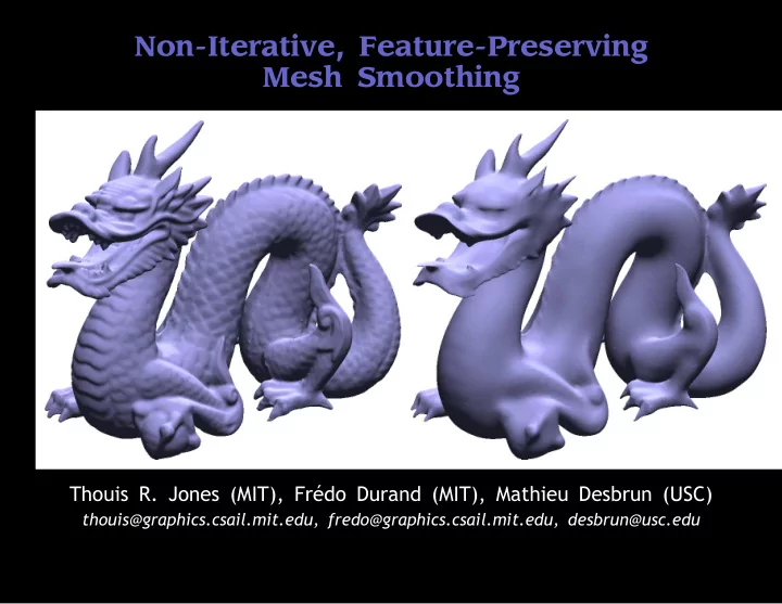
Non-Iterative, Feature-Preserving Mesh Smoothing Thouis R. Jones (MIT), Frédo Durand (MIT), Mathieu Desbrun (USC) thouis@graphics.csail.mit.edu, fredo@graphics.csail.mit.edu, desbrun@usc.edu

Why Smooth? 3D scanners are noisy... Jones, Durand, Desbrun

Why Smooth? 3D scanners are noisy... and have dropouts... Jones, Durand, Desbrun

Why Smooth? 3D scanners are noisy... and have dropouts... and usually require multiple scans. Jones, Durand, Desbrun

Goals Fast smoothing of meshes Robust • Geometrically: preserve features • Topologically: no connectivity information Simple to implement Jones, Durand, Desbrun

Goals Fast smoothing of meshes polygon soups Robust • Geometrically: preserve features • Topologically: no connectivity information Simple to implement Jones, Durand, Desbrun

Previous Work on Smoothing Fast Mesh Smoothing • Taubin 1995; Desbrun et al. 1999 Feature Preserving • Clarenz et al. 2000; Desbrun et al. 2000; Meyer et al. 2002; Zhang and Fiume 2002; Bajaj and Xu 2003 Diffusion on Normal Field • Taubin 2001; Belyaev and Ohtake 2001; Ohtake et al. 2002; Tasdizen et al. 2002 Wiener Filtering of Meshes • Peng et al. 2001; Alexa 2002; Pauly and Gross 2001 (points) Jones, Durand, Desbrun

Approach We cast feature-preserving filtering as a robust estimation problem on vertex positions. Extend Bilateral Filter to 3D. • Smith and Brady 1997; Tomasi and Manduchi 1998 Use first-order predictors based on facets of model. Single pass. Jones, Durand, Desbrun

Non-Robust Estimation Least Squares Error Norm 4 3 y 2 1 0 –2 –1 1 2 x Outliers have unlimited influence on estimate. Jones, Durand, Desbrun

Robust Estimation Robust Error Norm 0.3 0.25 0.2 y 0.15 0.1 0.05 0 –2 –1 1 2 x Outliers have bounded influence on estimate. Jones, Durand, Desbrun

Gaussian Filter (Non-robust) image spatial � ���� � �� � I ′ s = I ( p ) f ( s − p ) p I ′ I f Jones, Durand, Desbrun

Bilateral Filter (Robust) image spatial influence s = 1 � ���� � �� � � �� � I ′ I ( p ) f ( s − p ) g ( I s − I p ) k s p I ′ I f g fg Jones, Durand, Desbrun

Bilateral Filter (Robust) image spatial influence s = 1 � ���� � �� � � �� � I ′ I ( p ) f ( s − p ) g ( I s − I p ) k s p I ′ I f g fg Jones, Durand, Desbrun

Bilateral Filter (Robust) image spatial influence s = 1 � ���� � �� � � �� � I ′ I ( p ) f ( s − p ) g ( I s − I p ) k s p I ′ I f g fg Jones, Durand, Desbrun

Bilateral Filter (Robust) image spatial influence s = 1 � ���� � �� � � �� � I ′ I ( p ) f ( s − p ) g ( I s − I p ) k s p I ′ I f g fg Jones, Durand, Desbrun

Bilateral Filter (Robust) image spatial influence s = 1 � ���� � �� � � �� � I ′ I ( p ) f ( s − p ) g ( I s − I p ) k s p I ′ I f g fg Jones, Durand, Desbrun

Bilateral Filter (Robust) image spatial influence s = 1 � ���� � �� � � �� � I ′ I ( p ) f ( s − p ) g ( I s − I p ) k s p I ′ I f g fg Jones, Durand, Desbrun

Bilateral Filter (Robust) image spatial influence s = 1 � ���� � �� � � �� � I ′ I ( p ) f ( s − p ) g ( I s − I p ) k s p � k s = f ( s − p ) g ( I s − I p ) p Jones, Durand, Desbrun

Bilateral Filter Left: Jones and Jones 2003 Right: Bilaterally filtered. Jones, Durand, Desbrun

Extending the Bilateral Filter to Meshes How to separate location and signal in a 3D model? • Forming local frames requires a connected mesh. Instead, use first-order predictors based on facets: Π ( ) p q q p No connectivity required between facets. Jones, Durand, Desbrun

Bilateral Filter for Meshes Estimate p ′ , the new position for a vertex p prediction spatial influence area 1 � � �� � � �� � � �� � p ′ = ���� Π q ( p ) f ( || c q − p || ) g ( || Π q ( p ) − p || ) a q k ( p ) q ∈ S Jones, Durand, Desbrun

Bilateral Filter for Meshes Estimate p ′ , the new position for a vertex p prediction spatial influence area 1 � � �� � � �� � � �� � p ′ = ���� Π q ( p ) f ( || c q − p || ) g ( || Π q ( p ) − p || ) a q k ( p ) q ∈ S Jones, Durand, Desbrun

Bilateral Filter for Meshes Estimate p ′ , the new position for a vertex p prediction spatial influence area 1 � � �� � � �� � � �� � p ′ = ���� Π q ( p ) f ( || c q − p || ) g ( || Π q ( p ) − p || ) a q k ( p ) q ∈ S Jones, Durand, Desbrun

Bilateral Filter for Meshes Estimate p ′ , the new position for a vertex p prediction spatial influence area 1 � � �� � � �� � � �� � p ′ = ���� Π q ( p ) f ( || c q − p || ) g ( || Π q ( p ) − p || ) a q k ( p ) q ∈ S Jones, Durand, Desbrun

Why we expect it to work Predictions across corners are ``outliers''. Jones, Durand, Desbrun

Dealing with Noise Noise has a nonlinear effect on predictions. We must mollify (pre-smooth) normals. Jones, Durand, Desbrun

Dealing with Noise Noise has a nonlinear effect on predictions. We must mollify (pre-smooth) normals. Jones, Durand, Desbrun

Dealing with Noise Noise has a nonlinear effect on predictions. We must mollify (pre-smooth) normals. Jones, Durand, Desbrun

Dealing with Noise Noise has a nonlinear effect on predictions. We must mollify (pre-smooth) normals. Jones, Durand, Desbrun

Dealing with Noise Noise has a nonlinear effect on predictions. We must mollify (pre-smooth) normals. Jones, Durand, Desbrun

Implementation 3K vertices / second (typical), 1.4 GHz Athlon. Gaussians for f and g . Optimizations • Cutoff at twice spatial filter radius. • Binning for spatially coherent computation. Data and non-optimized code available online. Jones, Durand, Desbrun

Results - Smoothing Original Desbrun 1999 Our result Jones, Durand, Desbrun

Results - Effect of g Original Without g Our result Jones, Durand, Desbrun

Results - Effect of Mollification Original Without mollification Our result Jones, Durand, Desbrun

Results - Connectivity 50% Original Smoothed All predictors Jones, Durand, Desbrun

Results - Varying width of f and g Original Narrow spatial and influence Jones, Durand, Desbrun

Results - Varying width of f and g Original Narrow spatial and wide influence Jones, Durand, Desbrun

Results - Varying width of f and g Original Wide spatial and influence Jones, Durand, Desbrun

Normalization factor k as ``Confidence'' Normalization term k ( p ) is sum of weights, and is a measure of confidence in the estimation at p . 1 � p ′ = Π q ( p ) f ( || c q − p || ) g ( || Π q ( p ) − p || ) a q k ( p ) q ∈ S � k ( p ) = f ( || c q − p || ) g ( || Π q ( p ) − p || ) a q q ∈ S Jones, Durand, Desbrun

Results - k as Confidence Low High Jones, Durand, Desbrun

Results - k as Confidence Low High Jones, Durand, Desbrun

Results - vs Wiener Filtering Original Jones, Durand, Desbrun

Results - vs Wiener Filtering (Low Noise) Peng et al. 2001 Our result Jones, Durand, Desbrun

Results - vs Wiener Filtering (High Noise) Peng et al. 2001 Our result Jones, Durand, Desbrun

Results - vs Anisotropic Diffusion Original Jones, Durand, Desbrun

Results - vs Anisotropic Diffusion Clarenz et al. 2000 Our result Jones, Durand, Desbrun

Similar Methods Bilateral Mesh Denoising, Fleishman et al. 2003 (next talk) • Iterative • Local frame • No mollification • Different predictor Trilateral Filter, Cloudhury and Tumblin 2003 (EGSR) • Images and Meshes • Mollify normals, then vertices • Different predictor Jones, Durand, Desbrun

Future Work Extend to other types of data (point models, volume data). Using k to steer further processing. Iterative application. Jones, Durand, Desbrun

Conclusions Fast, feature preserving filter. Simple to implement. Applicable to polygon soups. Take-home message: • Robust estimation for smoothing. • Points across features are outliers. • First-order predictors remove connectivity requirements. Jones, Durand, Desbrun

Acknowledgements SIGGRAPH reviewers, Caltech SigDraft and MIT pre-reviewers. Udo Diewald, Martin Rumpf, Jianbo Peng, Denis Zorin, and Jean-Yves Bouguet, and Stanford 3D Scanning Repository for models. Peter Shirley and Michael Cohen for comments on this presentation. We would like to thank the NSF (CCR-0133983, DMS-0221666, DMS-0221669, EEC-9529152, EIA-9802220). Jones, Durand, Desbrun