
SLIDE 1
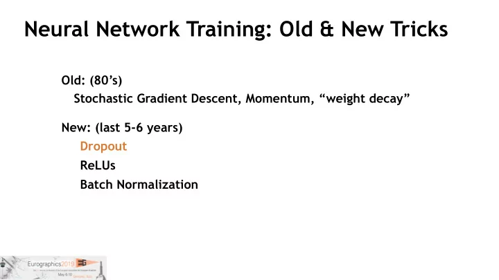
Stochastic Gradient Descent, Momentum, “weight decay” Dropout ReLUs Batch Normalization Old: (80’s) New: (last 5-6 years)
Neural Network Training: Old & New Tricks Old: (80s) Stochastic - - PowerPoint PPT Presentation
Neural Network Training: Old & New Tricks Old: (80s) Stochastic Gradient Descent, Momentum, weight decay New: (last 5-6 years) Dropout ReLUs Batch Normalization Reminder: Overfitting, in images Classification just right
Stochastic Gradient Descent, Momentum, “weight decay” Dropout ReLUs Batch Normalization Old: (80’s) New: (last 5-6 years)
2
Classification Regression
just right
3
Each sample is processed by a ‘decimated’ neural net
3
Each sample is processed by a ‘decimated’ neural net Decimated nets: distinct classifiers But: they should all do the same job
4
Stochastic Gradient Descent, Momentum, “weight decay” Dropout ReLUs Batch Normalization Old: (80’s) New: (last 5-6 years)
5
6
Sigmoidal (“logistic”) Rectified Linear Unit (RELU)
‘Neuron’: Cascade of Linear and Nonlinear Function
7
Outputs Reminder: a network in backward mode
7
Outputs
Gradient signal from above
Reminder: a network in backward mode
7
Outputs
Gradient signal from above
Reminder: a network in backward mode
7
Outputs
Gradient signal from above
Reminder: a network in backward mode
7
Outputs
Gradient signal from above scaling: <1 (actually <0.25)
Reminder: a network in backward mode
8
Gradient signal from above scaling: <1 (actually <0.25)
8
Gradient signal from above scaling: <1 (actually <0.25)
Do this 10 times: updates in the first layers get minimal Top layer knows what to do, lower layers “don’t get it” Sigmoidal Unit: Signal is not getting through!
9
Scaling: {0,1}
Gradient signal from above
10
Great! But… no gradient for negative half-space
10
Great! But… no gradient for negative half-space Lots of follow up work: LeakyReLU, eLU, etc. Can improve results, but typically fine-tuning only
Stochastic Gradient Descent, Momentum, “weight decay” Dropout ReLUs Batch Normalization Old: (80’s) New: (last 5-6 years)
11
12
10 am 2pm 7pm
13
Photometric transformation: I → a I + b
13
Photometric transformation: I → a I + b
13
Photometric transformation: I → a I + b
13
Photometric transformation: I → a I + b
13
Photometric transformation: I → a I + b
14
Whiten-as-you-go:
15
16
17
Example: 200x200 image 40K hidden units ~1.6B parameters!!!
Fully-connected Layer
18
Example: 200x200 image 40K hidden units Filter size: 10x10 4M parameters
Locally-connected Layer
Note: This parameterization is good when input image is registered (e.g., face recognition).
19
Note: This parameterization is good when input image is registered (e.g., face recognition). Example: 200x200 image 40K hidden units Filter size: 10x10 4M parameters
Locally-connected Layer
20
Share the same parameters across different locations (assuming input is stationary): Convolutions with learned kernels
Convolutional Layer
21
Convolutional Layer
22
Convolutional Layer
23
Convolutional Layer
24
Convolutional Layer
25
Convolutional Layer
26
Convolutional Layer
27
Convolutional Layer
28
Convolutional Layer
29
Convolutional Layer
30
Convolutional Layer
31
Convolutional Layer
32
Convolutional Layer
33
Convolutional Layer
34
Convolutional Layer
35
Convolutional Layer
36
Convolutional Layer
37
Fully-connected layer
#of parameters: K2
38
#of parameters: size of window
Convolutional layer
39
Convolutional layer
40
41
Learn multiple filters.
E.g.: 200x200 image 100 Filters Filter size: 10x10 10K parameters
Convolutional layer
42
Conv. layer
h1
n− 1
h2
n− 1
h3
n− 1
h1
n
h2
n
feature map input feature map kernel
Convolutional layer with ReLU activation
42
Conv. layer
h1
n− 1
h2
n− 1
h3
n− 1
h1
n
h2
n
feature map input feature map kernel
Convolutional layer with ReLU activation
ReLU
Activation
43
h1
n− 1
h2
n− 1
h3
n− 1
h1
n
h2
n
feature map input feature map kernel
Convolutional layer with ReLU activation
44
h1
n− 1
h2
n− 1
h3
n− 1
h1
n
h2
n
feature map input feature map kernel
Convolutional layer with ReLU activation
45
De-convolutional layer with ReLU activation
De-conv. layer
h1
n− 1
h2
n− 1
h3
n−
h1
n
h2
n
Still holds, same structure
45
De-convolutional layer with ReLU activation
No real inverse - but convolutions can easily go the other way
De-conv. layer
h1
n− 1
h2
n− 1
h3
n−
h1
n
h2
n
Still holds, same structure
45
De-convolutional layer with ReLU activation
No real inverse - but convolutions can easily go the other way
De-conv. layer
h1
n− 1
h2
n− 1
h3
n−
h1
n
h2
n
“De-convolution” or “Transposed convolution”
Still holds, same structure
45
De-convolutional layer with ReLU activation
No real inverse - but convolutions can easily go the other way
De-conv. layer
h1
n− 1
h2
n− 1
h3
n−
h1
n
h2
n
“De-convolution” or “Transposed convolution” Also a convolution with transposed weight tensor
Still holds, same structure
46
Pooling layer
47
Pooling layer
48
Pooling layer: receptive field size
49
Pooling layer: receptive field size
50
51
52
53
54
55
56
57
58
59
60
INPUT 32x32
Convolutions Subsampling Convolutions
C1: feature maps 6@28x28
Subsampling
S2: f. maps 6@14x14 S4: f. maps 16@5x5 C5: layer 120 C3: f. maps 16@10x10 F6: layer 84
Full connection Full connection Gaussian connections
OUTPUT 10
Gradient-based learning applied to document recognition, Y . LeCun, L. Bottou, Y . Bengio, and P . Haffner, 1998.
https://www.youtube.com/watch?v=FwFduRA_L6Q
61
61
deep learning = neural networks (+ big data + GPUs)
61
deep learning = neural networks (+ big data + GPUs) + a few more recent tricks!
AlexNet Alex Krizhevsky, Ilya Sutskever, Geoffrey E. Hinton: ImageNet classification with deep convolutional neural
62
VGG Karen Simonyan, Andrew Zisserman (=Visual Geometry Group) Very Deep Convolutional Networks for Large-Scale Image Recognition, arxiv, 2014.
63
ResNet Kaiming He, Xiangyu Zhang, Shaoqing Ren, Jian Sun, Deep Residual Learning for Image Recognition, CVPR 2016.
64
65
66
67
68
Some Network residual Preserving base information can treat perturbation
69
Appropriate for treating perturbation as keeping a base information
70
71
72
73
Densely Connected Convolutional Networks, CVPR 2017 Gao Huang, Zhuang Liu, Laurens van der Maaten, Kilian Q. Weinberger Recently proposed, better performance/parameter ratio
74
75
76
77
78
79
80
81
32-fold decimation 224x224 to 7x7
82
83
Space Space Features
84
85
U-Net: Convolutional Networks for Biomedical Image Segmentatio. Ronneberger et al. 2015
SIGGRAPH Asia Course CreativeAI: Deep Learning for Graphics
86
87
88
89
89
standard
89
standard standard
89
standard standard history, stored data
89
standard standard history, stored data weight new vs. stored data
89
standard standard history, stored data weight new vs. stored data forget stored data
89
standard standard history, stored data weight new vs. stored data forget stored data control amount of data output
90
[Sutskever et al., “Sequence to Sequence Learning with Neural Networks”, 2014]
91
[Bai et al., "An empirical evaluation of generic convolutional and recurrent networks for sequence modeling”, 2018] [Chung et al., "Empirical evaluation of gated recurrent neural networks on sequence modeling”,2014]
92
(Python) (Python, C++, Java) (C++, Python, Matlab) (Python, backends support other languages)
(Python, C++, C#) (Python, C++, and others) (Matlab) (Python, Java, Scala) (Python) (Python, C++) (Python)
Google Trends for search terms: “[name] tutorial” Google Trends for search terms: “[name] github”
for i = 1 .. max_iterations input, ground_truth = load_minibatch(data, i)
loss = compute_loss(output, ground_truth) # gradients of loss with respect to parameters gradients = network_backpropagate(loss, parameters) parameters = optimizer_step(parameters, gradients)
feature channels C spatial width W spatial height H batches B
4D convolution kernel: OC x IC x KH x KW 4D input data: B x C x H x W
input channels IC kernel height KH kernel width KW
OC
parameters = (weight, bias)
loss = (output - ground_truth)^2 # gradients of loss with respect to parameters gradients = backpropagate(loss, parameters)
weight input bias
+ *
ground_truth
2 loss
σ
𝑝1 𝑝2 𝑝3
+ *
𝜖 loss 𝜖 weight
loss
σ
𝜖 loss 𝜖 bias 𝜖 loss 𝜖 𝑝1 𝜖 loss 𝜖 𝑝2 𝜖 loss 𝜖 output 𝜖 loss 𝜖 𝑝3
forward pass backward pass
Since loss is a scalar, the gradients are the same size as the parameters
𝑔
inputs
𝑔
𝜖 loss 𝜖 parameters 𝜖 loss 𝜖 inputs 𝜖 loss 𝜖 outputs
parameters , = backward()
define once, evaluate during training define implicitly by running operations, a new graph is created in each evaluation
x = Variable() loss = if_node(x < parameter[0], x + parameter[0], x - parameter[1]) for i = 1 .. max_iterations x = data() run(loss) backpropagate(loss, parameters) for i = 1 .. max_iterations x = data() if x < parameter[0] loss = x + parameter[0] else loss = x – parameter[1] backpropagate(loss, parameters)
convertor tensorflow pytorch keras caffe caffe2 CNTK chainer mxnet tensorflow
MMdnn model-converters/ nn_toolsconvert-to- tensorflow/MMdnn MMdnn/ nn_tools None crosstalk/MMdnn None MMdnn pytorch pytorch2keras (over Keras)
nn-transfer Pytorch2caffe/ pytorch-caffe- darknet-convert
ONNX None None keras nn_tools /convert-to- tensorflow/ keras_to_tensorflow/ keras_to_tensorflow/ MMdnn MMdnn/ nn-transfer
None MMdnn None MMdnn caffe MMdnn/nn_tools/ caffe-tensorflow MMdnn/ pytorch-caffe- darknet- convert/ pytorch-resnet caffe_weight_converter / caffe2keras/nn_tools/ kerascaffe2keras/ Deep_Learning_Model_ Converter/MMdnn
crosstalkcaffe/ CaffeConverterMMdnn None mxnet/tools/ caffe_converter/ ResNet_caffe2mxnet/ MMdnn caffe2 None ONNX None None
None None CNTK MMdnn ONNX MMdnn MMdnn MMdnn ONNX
MMdnn chainer None chainer2pytorc h None None None None
mxnet MMdnn MMdnn MMdnn MMdnn/MXNet2Caffe/ Mxnet2Caffe None MMdnn None
development for Pytorch, Caffe2, Chainer, CNTK, and MxNet
Tensorflow
available for several frameworks
representation, but no clear standard
SIGGRAPH Asia Course CreativeAI: Deep Learning for Graphics
107