Network Tomography for Fault Diagnosis Renata Teixeira CNRS and - - PDF document

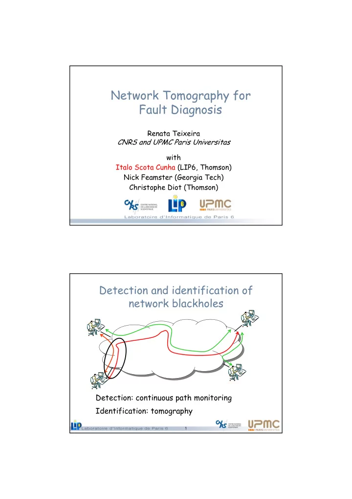
Network Tomography for Fault Diagnosis

Renata Teixeira CNRS and UPMC Paris Universitas with Italo Scota Cunha (LIP6, Thomson) Nick Feamster (Georgia Tech) Christophe Diot (Thomson)

1

Detection and identification of network blackholes

Detection: continuous path monitoring Identification: tomography

2

Problem: Too many false alarms

Applying tomography on raw measurements

– PlanetLab: one alarm per minute – Thomson VPN: one alarm every two minutes

Why?

– Loss can be transient, topology can change – Different monitors see different conditions

Detection: transient losses vs. persistent failures

Monitors ping a set of destinations Lost pings can have different causes

Congestion Routing changes Persistent failures

How to know which losses are persistent?

3

4

Failure confirmation

time loss burst packets on a path

Upon detection of a failure, trigger extra probes Goal: minimize detection errors

Detection error

5

Probing strategy for failure confirmation

Which probing process?

– Assume link losses follow a Gilbert process – Periodic probing minimizes detection errors

How many probes?

– Confirm failures with a target detection-error rate – Assume independence and a given a loss rate

How much time between probes?

– Reduce chance that probes fall on the same loss burst

Tradeoff: detection error and detection time

Identification through binary tomography

6

Given: topology and end-to-end path statuses Find the smallest set of links that explain observations

m t1 t2

Lack of synchronization leads to inconsistencies

Inconsistent measurements: Different monitors see different conditions

Achieving consistency: Aggregation strategies

Basic strategy

– Waits for one cycle

Multi-Cycle strategy (MC)

– Waits for n cycles with identical path statuses

Per-Path Multi-Cycle strategy (MC-path)

– Only considers paths that are down for n cycles

9

Evaluation

Evaluation is challenging

– Need ground truth and realistic environment

Analytic modeling – Understand limits of the system Controlled Experiments: Emulab testbed – Realistic environment – Control over failures Wide-area Experiments: PlanetLab, Thomson

– Real losses and failures, but no ground truth

Failure confirmation reduces false alarms

10

Emulab experiments with 0.6% detection errors

Aggregation strategies identify most long failures

Emulab experiments with 0.6% detection errors

12

Emulab experiments with 0.6% detection errors

Multi-cycle aggregation reduces false alarms Number of alarms in wide-area experiments

13

PlanetLab Thomson

Thomson

– 56 paths – Cycles: 5 seconds

PlanetLab

– 39,800 paths – Cycles: 60 seconds

Summary

Tomography with raw data leads to false alarms Two techniques to reduce false alarms

– Failure confirmation

• Distinguishes transient losses and persistent

– Aggregation

• Combines measurements from different monitors

14

Two deployment scenarios

15