Negative Gearing and Welfare: A Quantitative Study of the Australian - - PowerPoint PPT Presentation

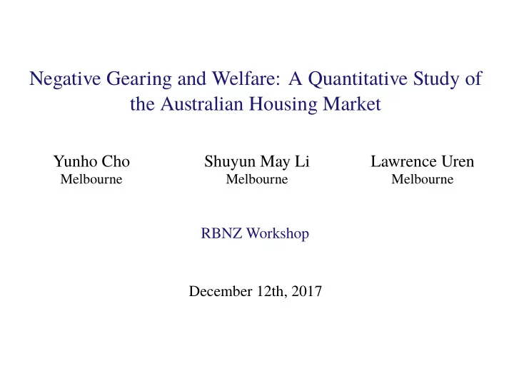
Negative Gearing and Welfare: A Quantitative Study of the Australian Housing Market

Yunho Cho

Melbourne

Shuyun May Li

Melbourne

Lawrence Uren

Melbourne

RBNZ Workshop December 12th, 2017

“We haven’t got any plans to review the policy (negative gearing) we took to the

• election. Can I just say to you that the issue of housing affordability is
• verwhelmingly a question of supply.”

Malcolm Turnbull, PM of Australia “... deep down in the core of the Turnbull government, they know that if they want to resuscitate the Australian dream of owning your own home, they need to act on negative gearing.” Bill Shorten, Opposition Leader

Negative gearing in Australian housing market

• Negative gearing: Landlords deduct housing investment losses from gross

income at their marginal rates

Figures: Negative Gearing

1

Negative gearing in Australian housing market

• Negative gearing: Landlords deduct housing investment losses from gross

income at their marginal rates

Figures: Negative Gearing

• Arguments for

– facilitate construction of new houses – stimulate supply of rental housing – help renters with affordable shelter services

• Arguments against

– most housing investment is to purchase established properties – possibly worsen inequality – additional upward pressure on house prices

1

This paper

• Question: What are the welfare implications of negative gearing for

heterogeneous Australian households?

2

This paper

• Question: What are the welfare implications of negative gearing for

heterogeneous Australian households?

• Model: General equilibrium OLG model with incomplete markets and

heterogeneous agents

– uninsurable idiosyncratic income shock – endogenous house prices and rents – income tax code and negative gearing for housing investment

2

This paper

• Question: What are the welfare implications of negative gearing for

heterogeneous Australian households?

• Model: General equilibrium OLG model with incomplete markets and

heterogeneous agents

– uninsurable idiosyncratic income shock – endogenous house prices and rents – income tax code and negative gearing for housing investment

• Calibrate: Match life-cycle profiles from micro-data and moments of

Australian housing market

• Simulate: Compare stationary equilibria with and without negative

gearing

2

Main findings

Repealing negative gearing

• Improves housing affordability and increases homeownership rate

– lower house prices and higher rents ⇒ lower price-to-rent ratio

• Reduces housing investment

– aggregate rental supply and landlord rate fall – most of young landlords with high earning driven out of the market

3

Main findings

Repealing negative gearing

• Improves housing affordability and increases homeownership rate

– lower house prices and higher rents ⇒ lower price-to-rent ratio

• Reduces housing investment

– aggregate rental supply and landlord rate fall – most of young landlords with high earning driven out of the market

• Overall welfare gain of 1.5% and 76% of households better off

– redistribution plays a key role for welfare gain – with redistribution, renters are winners and landlords are losers

3

Model

Demographics

• Unit-mass of finitely-lived households
• Live and work for a = 1, 2, ..., 14 periods

– the model period is 5 years – households enter the economy at age 21 and exit at age 90

• Age-dependent survival rate, κa with κ14 = 0

4

Preferences

• Expected life-time utility of household

E0 14

• a=1

βa−1κaua(ca, ˜ ha)

• ,

β ∈ (0, 1) c: non-durable consumption; ˜ h: housing services

• Utility function

ua(c, ˜ h) =

• cα(λ˜

h)

1−α1−σ

1−σ

, α, σ ∈ [0, ∞) λ > 1 for homeowners; λ = 1 for renters

5

Preferences

• Expected life-time utility of household

E0 14

• a=1

βa−1κaua(ca, ˜ ha)

• ,

β ∈ (0, 1) c: non-durable consumption; ˜ h: housing services

• Utility function

ua(c, ˜ h) =

• cα(λ˜

h)

1−α1−σ

1−σ

, α, σ ∈ [0, ∞) λ > 1 for homeowners; λ = 1 for renters

• Accidental bequest: assets of deceased households equally distributed to

surviving households

5

Housing

• Housing services ˜

h can be obtained by purchasing or renting

• Households can buy at price p or rent at pr per unit
• Households become

– landlords if h > ˜ h > 0 – owner-occupiers if h = ˜ h > 0 – renters if ˜ h > h = 0

• Renters can live in houses that are smaller than the minimum housing size

available to homeowners

• No renter-landlords

6

Housing as risky asset

• Sales of housing asset subject to idiosyncratic house price shock ω ∈ Ω
• Ex-ante expected capital gain is zero ⇒ E(ωp) = p
• ω not realized until house is sold

– households know unconditional probability of the shock πω

7

Housing as risky asset

• Sales of housing asset subject to idiosyncratic house price shock ω ∈ Ω
• Ex-ante expected capital gain is zero ⇒ E(ωp) = p
• ω not realized until house is sold

– households know unconditional probability of the shock πω

• Competitive construction firm buys from selling households and sell old

and new houses to purchasing households at price p

7

Maintenance and transaction costs

• Homeowners bear maintenance expense at constant rate δ
• Landlords incur additional (fixed) expense ζ
• Linear transaction costs

TC(h−1, h) = if h−1 = h φbph + φs(ωp)h−1 if h−1 = h

8

Borrowing and saving

• Households can save by holding a risk-free asset s′ > 0 that pays interest r
• Households can borrow s′ < 0, subject to a collateral constraint

s′ ≥ −(1 − θ)ph

• Borrowing also requires

– downpayment θ – interest payment at rate r + m

9

Taxation and transfers

• Net rental income

NRI ≡

• (pr − pδ)(h − ˜

h) − ζ + (r + m)s

• h−˜

h h

• I{s<0}
• I{h>˜

h} 10

Taxation and transfers

• Net rental income

NRI ≡

• (pr − pδ)(h − ˜

h) − ζ + (r + m)s

• h−˜

h h

• I{s<0}
• I{h>˜

h}

• Total taxable income

Y = ya + rsI{s>0} + NRI

• If NRI < 0, negative gearing applies

10

Taxation and transfers

• Net rental income

NRI ≡

• (pr − pδ)(h − ˜

h) − ζ + (r + m)s

• h−˜

h h

• I{s<0}
• I{h>˜

h}

• Total taxable income

Y = ya + rsI{s>0} + NRI

• If NRI < 0, negative gearing applies
• Counter-factual policy experiment by setting

Y = ya + rsI{s>0} + NRII{NRI>0}

• Progressive income tax system
• Receive lump-sum transfers F

10

Government and construction sector

• Government collects tax T(Y ), sells assets of deceased households R, and

distributes lump-sum transfers F

11

Government and construction sector

• Government collects tax T(Y ), sells assets of deceased households R, and

distributes lump-sum transfers F

• Competitive construction firm

– buys existing houses from selling households – develops unoccupied land L at constant price – sells old and new houses at market price p

11

Government and construction sector

• Government collects tax T(Y ), sells assets of deceased households R, and

distributes lump-sum transfers F

• Competitive construction firm

– buys existing houses from selling households – develops unoccupied land L at constant price – sells old and new houses at market price p

• Solves static problem

Hnew = maxL

• pψ1Lψ2 − L
• which gives the law of motion for the aggregate housing supply

H = H−1(1 − δ) + Hnew

• Housing supply elasticity given by ε =

ψ2 1−ψ2 ∈ [0, ∞) 11

Parameterization overview

• Earnings process estimated from the HILDA survey

– gross income that includes pensions and other social benefits but excludes any investment income

• Tax function calibrated to the current Australian income tax system
• House price shock quantified from the SIH
• Discretize state space for housing

h ∈ {h(1), ..., h(K)} hrent ∈ {hrent(1), ..., hrent(J), h(1), ..., h(K)}

• Preference parameters and landlord fixed cost calibrated internally

12

Model fit

• Homeownership and landlord rates over life-cycle and income quintiles

13

Simulation

Steady state

Baseline No NG ε = 2 Price 1.180 1.160 Rent 0.164 0.168 Price-rent ratio 7.209 6.907

• Frac. of homeowners
• Frac. of owner-occupiers
• Frac. of landlords
• Frac. of renters

Rental supply (relative to housing supply) Aggregate housing supply (normalized) Transfers Debt to income ratio

14

Steady state

Baseline No NG ε = 2 Price 1.180 1.160 Rent 0.164 0.168 Price-rent ratio 7.209 6.907

• Frac. of homeowners

0.667 0.722

• Frac. of owner-occupiers

0.500 0.584

• Frac. of landlords

0.167 0.138

• Frac. of renters

0.333 0.278 Rental supply (relative to housing supply) Aggregate housing supply (normalized) Transfers Debt to income ratio

14

Steady state

Baseline No NG ε = 2 Price 1.180 1.160 Rent 0.164 0.168 Price-rent ratio 7.209 6.907

• Frac. of homeowners

0.667 0.722

• Frac. of owner-occupiers

0.500 0.584

• Frac. of landlords

0.167 0.138

• Frac. of renters

0.333 0.278 Rental supply (relative to housing supply) 0.263 0.184 Aggregate housing supply (normalized) 1 0.987 Transfers Debt to income ratio

14

Steady state

Baseline No NG ε = 2 Price 1.180 1.160 Rent 0.164 0.168 Price-rent ratio 7.209 6.907

• Frac. of homeowners

0.667 0.722

• Frac. of owner-occupiers

0.500 0.584

• Frac. of landlords

0.167 0.138

• Frac. of renters

0.333 0.278 Rental supply (relative to housing supply) 0.263 0.184 Aggregate housing supply (normalized) 1 0.987 Transfers 0.229 0.236 Debt to income ratio 0.356 0.304

14

∆ in homeownership and landlord rates

15

Welfare Analysis

Welfare criterion

• Consumption equivalent variation (CEV)

– percentage change in current consumption of non-durables that equates expected discount utility in counterfactual vs. baseline

16

Welfare criterion

• Consumption equivalent variation (CEV)

– percentage change in current consumption of non-durables that equates expected discount utility in counterfactual vs. baseline

• Formally

V nong(x) =

• ω∈Ω
• πω
• u
• c∗

ω(x) + cev, ˜

h∗

ω(x)

• + βκaEz′|zV ng(x′∗

ω (x))

• for any x ≡ (a, s, h−1, z)

c∗

ω(x), ˜

h∗

ω(x), x′∗ ω (x): optimal decision rules in baseline economy 16

Welfare criterion

• Consumption equivalent variation (CEV)

– percentage change in current consumption of non-durables that equates expected discount utility in counterfactual vs. baseline

• Formally

V nong(x) =

• ω∈Ω
• πω
• u
• c∗

ω(x) + cev, ˜

h∗

ω(x)

• + βκaEz′|zV ng(x′∗

ω (x))

• for any x ≡ (a, s, h−1, z)

c∗

ω(x), ˜

h∗

ω(x), x′∗ ω (x): optimal decision rules in baseline economy

• Positive CEV ⇒ the household better off in counterfactual economy

16

Welfare: price vs. redistribution effects

Simulate counterfactual economy under two scenarios:

• 1. No negative gearing without redistribution (price effect)

– keep the same transfer payment to baseline economy

• 2. No negative gearing with redistribution (redistribution effect)

– the government distributes all its revenue

17

Welfare: price vs. redistribution effects

Simulate counterfactual economy under two scenarios:

• 1. No negative gearing without redistribution (price effect)

– keep the same transfer payment to baseline economy

• 2. No negative gearing with redistribution (redistribution effect)

– the government distributes all its revenue

Note: There are no price and quantity differences across the steady states

17

Redistribution key channel for welfare gain

Mean CEV Median CEV P(CEV > 0) Price effect

• 0.026
• 0.007

0.325 Redistribution effect 0.015 0.047 0.756

18

Welfare effects by housing tenure

Initial Housing Tenure Mean CEV Median CEV P(CEV > 0) Renter 0.049 0.051 0.776 Owner-occupier

• 0.015

0.036 0.776 Landlord

• 0.099
• 0.018

0.455

19

Welfare effects by housing tenure and income

Median CEV Initial Housing Income Quintile Tenure Q1 Q2 Q3 Q4 Q5 Renter 0.059 0.057 0.051 0.049 0.053 Owner-occupier 0.025 0.036 0.036 0.037 0.039 Landlord 0.027 0.009

• 0.014
• 0.072
• 0.363

P(CEV > 0) Initial Housing Income Quintile Tenure Q1 Q2 Q3 Q4 Q5 Renter 0.812 0.782 0.732 0.915 0.944 Owner-occupier 0.672 0.704 0.782 0.788 0.858 Landlord 0.718 0.544 0.475 0.374 0.106 20

Summary

• Built a quantitative model to explore the effects of negative gearing tax on

welfare of Australian households

21

Summary

• Built a quantitative model to explore the effects of negative gearing tax on

welfare of Australian households

• What have we learned from the model?

Removing negative gearing would

• 1. decrease house prices, (marginally) increase rents ⇒ improve housing

affordability

• 2. increase homeownership rate ⇒ shifting from renting to owning
• 3. reduce housing investment
• 4. welfare improves and most households would be better off
• 5. with redistribution, renters are winners, landlords especially young with high

earnings are losers

21

Figure: Negatively geared housing investors (left); Total rental income (right)

Source: Taxation Statistics, Australian Taxation Office

Go back