natural language processing classification
play

Natural Language Processing Classification Classification III Dan - PDF document

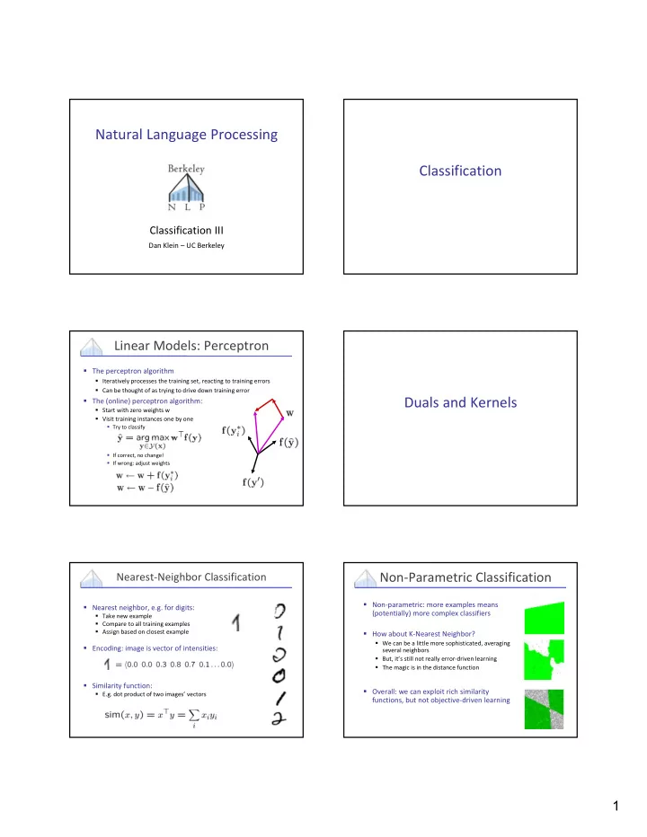
Natural Language Processing Classification Classification III Dan Klein UC Berkeley Linear Models: Perceptron The perceptron algorithm Iteratively processes the training set, reacting to training errors Can be thought of as trying


  1. Natural Language Processing Classification Classification III Dan Klein – UC Berkeley Linear Models: Perceptron  The perceptron algorithm  Iteratively processes the training set, reacting to training errors  Can be thought of as trying to drive down training error Duals and Kernels  The (online) perceptron algorithm:  Start with zero weights w  Visit training instances one by one  Try to classify  If correct, no change!  If wrong: adjust weights Non ‐ Parametric Classification Nearest ‐ Neighbor Classification  Non ‐ parametric: more examples means  Nearest neighbor, e.g. for digits: (potentially) more complex classifiers  Take new example  Compare to all training examples  Assign based on closest example  How about K ‐ Nearest Neighbor?  We can be a little more sophisticated, averaging  Encoding: image is vector of intensities: several neighbors  But, it’s still not really error ‐ driven learning  The magic is in the distance function  Similarity function:  Overall: we can exploit rich similarity  E.g. dot product of two images’ vectors functions, but not objective ‐ driven learning 1

  2. A Tale of Two Approaches… The Perceptron, Again  Nearest neighbor ‐ like approaches  Start with zero weights  Work with data through similarity functions  Visit training instances one by one  Try to classify  No explicit “learning”  Linear approaches  Explicit training to reduce empirical error  If correct, no change!  If wrong: adjust weights  Represent data through features  Kernelized linear models  Explicit training, but driven by similarity!  Flexible, powerful, very very slow mistake vectors Perceptron Weights Dual Perceptron   What is the final value of w? Track mistake counts rather than weights  Can it be an arbitrary real vector? Start with zero counts (  )   No! It’s built by adding up feature vectors (mistake vectors).  For each instance x  Try to classify mistake counts  If correct, no change!  If wrong: raise the mistake count for this example and prediction  Can reconstruct weight vectors (the primal representation) from update counts (the dual representation) for each i Dual / Kernelized Perceptron Issues with Dual Perceptron  Problem: to score each candidate, we may have to compare  How to classify an example x? to all training candidates  Very, very slow compared to primal dot product!  One bright spot: for perceptron, only need to consider candidates we made mistakes on during training  Slightly better for SVMs where the alphas are (in theory) sparse  This problem is serious: fully dual methods (including kernel methods) tend to be extraordinarily slow  Of course, we can (so far) also accumulate our weights as we go...  If someone tells us the value of K for each pair of candidates, never need to build the weight vectors 2

  3. Kernels: Who Cares? Some Kernels  So far: a very strange way of doing a very simple  Kernels implicitly map original vectors to higher dimensional calculation spaces, take the dot product there, and hand the result back  Linear kernel:  “Kernel trick”: we can substitute any* similarity function in place of the dot product  Quadratic kernel:  Lets us learn new kinds of hypotheses  RBF: infinite dimensional representation * Fine print: if your kernel doesn’t satisfy certain technical requirements, lots of proofs break.  Discrete kernels: e.g. string kernels, tree kernels E.g. convergence, mistake bounds. In practice, illegal kernels sometimes work (but not always). Tree Kernels [Collins and Dual Formulation for SVMs Duffy 01]  We want to optimize: (separable case for now)  This is hard because of the constraints  Solution: method of Lagrange multipliers  Want to compute number of common subtrees between T, T’  The Lagrangian representation of this problem is:  Add up counts of all pairs of nodes n, n’  Base: if n, n’ have different root productions, or are depth 0:  Base: if n, n’ are share the same root production:  All we’ve done is express the constraints as an adversary which leaves our objective alone if we obey the constraints but ruins our objective if we violate any of them Lagrange Duality Dual Formulation II  We start out with a constrained optimization problem:  Duality tells us that  We form the Lagrangian: has the same value as  This is useful because the constrained solution is a saddle point of  (this is a general property): This is useful because if we think of the  ’s as constants, we have an  unconstrained min in w that we can solve analytically.  Then we end up with an optimization over  instead of w (easier). Primal problem in w Dual problem in  3

  4. Dual Formulation III Back to Learning SVMs  Minimize the Lagrangian for fixed  ’s:  We want to find  which minimize  This is a quadratic program:  Can be solved with general QP or convex optimizers  So we have the Lagrangian as a function of only  ’s:  But they don’t scale well to large problems  Cf. maxent models work fine with general optimizers (e.g. CG, L ‐ BFGS)  How would a special purpose optimizer work? Coordinate Descent I Coordinate Descent II  Ordinarily, treating coordinates independently is a bad idea, but here the update is very fast and simple  Despite all the mess, Z is just a quadratic in each  i (y)  Coordinate descent: optimize one variable at a time  So we visit each axis many times, but each visit is quick  This approach works fine for the separable case  For the non ‐ separable case, we just gain a simplex constraint and so we need slightly more complex methods (SMO, exponentiated gradient) 0 0  If the unconstrained argmin on a coordinate is negative, just clip to zero… What are the Alphas?  Each candidate corresponds to a primal constraint Structure  In the solution, an  i (y) will be: Support vectors  Zero if that constraint is inactive  Positive if that constrain is active  i.e. positive on the support vectors  Support vectors contribute to weights: 4

  5. Handwriting recognition CFG Parsing x y x y brace The screen was a sea of red Sequential structure Recursive structure [Slides: Taskar and Klein 05] Bilingual Word Alignment Structured Models En x y vertu de les What nouvelle space of feasible outputs What is the anticipated is propositions the cost of collecting fees , anticipated under the new proposal? quel Assumption: cost est of le collecting En vertu de nouvelle côut fees prévu propositions, quel est le under de côut prévu de perception the perception de les droits? new de proposal le Score is a sum of local “part” scores ? droits ? Parts = nodes, edges, productions Combinatorial structure CFG Parsing Bilingual word alignment En # (NP  DT NN) vertu de What les … is nouvelle the k propositions # (PP  IN NP) anticipated ,  association cost quel of est …  position collecting le fees côut # (NN  ‘sea’) under  orthography prévu the de new perception j proposal de ? le droits ? 5

  6. [e.g. Option 0: Reranking Charniak and Reranking Johnson 05] Input N-Best List Output  Advantages: (e.g. n=100)  Directly reduce to non ‐ structured case  No locality restriction on features x = Baseline Non-Structured “The screen was a sea of red.” Parser Classification  Disadvantages:  Stuck with errors of baseline parser …  Baseline system must produce n ‐ best lists  But, feedback is possible [McCloskey, Charniak, Johnson 2006] Efficient Primal Decoding Structured Margin   Remember the margin objective: Common case: you have a black box which computes at least approximately, and you want to learn w  Many learning methods require more (expectations, dual representations,  This is still defined, but lots of constraints k ‐ best lists), but the most commonly used options do not  Easiest option is the structured perceptron [Collins 01]  Structure enters here in that the search for the best y is typically a combinatorial algorithm (dynamic programming, matchings, ILPs, A*…)  Prediction is structured, learning update is not Full Margin: OCR Parsing example  We want:  We want: S “brace” ‘I t was red’ A B C D  Equivalently:  Equivalently: S S “brace” “aaaaa” ‘I t was red’ ‘I t was red’ A B A B D F C D S S “brace” “aaaab” A B A B ‘I t was red’ ‘I t was red’ C D C D a lot! a lot! … … S S “brace” “zzzzz” A B E F ‘I t was red’ ‘I t was red’ C D G H 6

Download Presentation
Download Policy: The content available on the website is offered to you 'AS IS' for your personal information and use only. It cannot be commercialized, licensed, or distributed on other websites without prior consent from the author. To download a presentation, simply click this link. If you encounter any difficulties during the download process, it's possible that the publisher has removed the file from their server.

Recommend


More recommend