
SLIDE 1
Multi-Layered Perceptrons (MLPs)
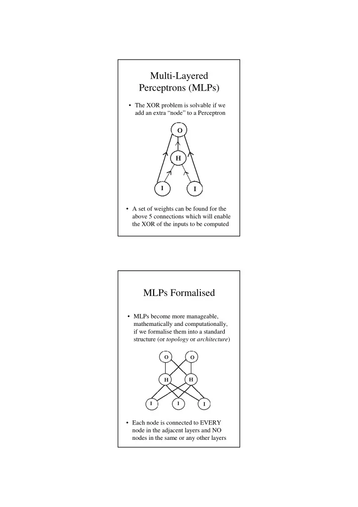
- A set of weights can be found for the
above 5 connections which will enable the XOR of the inputs to be computed
- The XOR problem is solvable if we
add an extra “node” to a Perceptron
MLPs Formalised
- Each node is connected to EVERY
node in the adjacent layers and NO nodes in the same or any other layers
- MLPs become more manageable,