Morse Parameters of -Uranium by Ab-initio Calculation Hyun Woo Seong - - PDF document

Morse Parameters of α-Uranium by Ab-initio Calculation

Hyun Woo Seonga, Ho Jin Ryu a,

a Department of Nuclear & Quantum Engineering, Korea Advanced Institute of Science and Technology, 291

Daehakro, Yuseong, 34141, Republic of Korea

*Corresponding author: hojinryu@kaist.ac.kr

• 1. Introduction

Uranium oxide fuels are mainly used in conventional nuclear power reactors. Nowadays, uranium alloys are actively being developed for fast reactors and research reactors [1-4]. For fuel design, the effects of radiation damage on the fuel performance should be considered. However, there are limitation to the experiments of radioactive materials. Computer simulation can help to

• vercome these limitations.

Molecule dynamics (MD) is widely used to predict material properties and structures, understand the atomic motion and identify a mechanism in chemical reactions. There are two types of MD; ab-initio MD and classical

• MD. Ab-initio MD provides accurate and reliable results.

However, it is affected by the system size and timescale. Only hundreds of atoms and several picoseconds are generally calculated. On the other hand, classical MD is suitable for large scale calculations such as plastic deformation and radiation damage. However, the accuracy of classical MD is dependent on interatomic potentials. There are many types of interatomic potentials. Many body potentials such as embedded atom method (EAM) [5,6] and modified embedded atom method (MEAM) [7] are usually used for alloys. However, the many body potentials exist only in popular materials and to development of new many body potentials is

• complicated. When proper many body potentials do not

exist, Morse potentials can be used instead of many-body

• potentials. There are applications of the Morse potential

function to cubic structure metals. However, there is no application to orthogonal structure such as α-uranium. In this study, we obtained Morse potential function of α- uranium using the result of ab-initio and analyze the reliability by comparing it to the existing potentials of uranium [8,9].

• 2. Methods and Results

The details of ab-initio and results of ab-initio are described in Section 2.1. In 2.2 section, the theory of Morse potential is described and Morse parameters are

• described. The results of MD simulation with Morse

potential and previous potentials of uranium are described and compared in Section 2.3. 2.1 Ab-initio calculation Ab-initio calculation is based on density functional theory(DFT) which is implemented in the Vienna ab initio Simulation Package (VASP) [10,11]. The plane- wave basis set with an energy cutoff of 550eV within the framework of the projector augmented wave (PAW) method [12,13] is used to describe the valence electrons. The exchange-correlation functional parameterized in the generalized gradient approximation (GGA) [14] by Perdew, Burke, and Emzerhof (PBE) [15] is used. We treat 6s26p67s25f36d1 as valence electrons for α-U. A Monkhorst-Pack k-points grid [16] is used for sampling

• f the Brillouin zone, with an 18×9×11 mesh. The partial
• ccupancies are set using the Methfessel-Paxton method

[17] of order one with a smearing width of 0.2 eV. The electronic and ionic optimizations are performed using a Davidson-block algorithm [18] and a Conjugate-gradient algorithm [19], respectively. The stopping criteria for self-consistent loops are 0.1 meV/cell and 1 meV/cell tolerance of total energy for the electronic and ionic relaxation, respectively. Bulk modulus is calculated by elastic constants. Elastic constants are calculated as the displacement of all atoms by 0.015 Å with x, y, and z

• direction. The rotationally invariant DFT + U method

introduced by Dudarev et al. [20], Eq. (2.5) is used for 5f3 electrons in α-U with Ueff = 1.24 eV [21] and Ueff = 1eV.

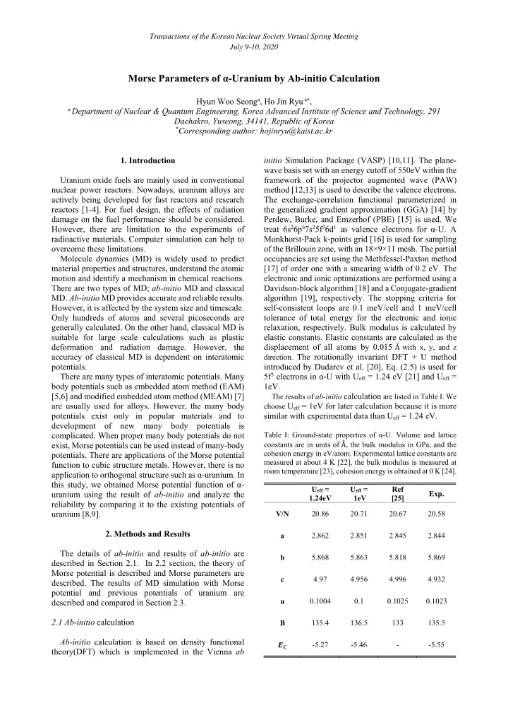
The results of ab-initio calculation are listed in Table I. We choose Ueff = 1eV for later calculation because it is more

similar with experimental data than Ueff = 1.24 eV.

Table I: Ground-state properties of α-U. Volume and lattice constants are in units of Å, the bulk modulus in GPa, and the cohesion energy in eV/atom. Experimental lattice constants are measured at about 4 K [22], the bulk modulus is measured at room temperature [23], cohesion energy is obtained at 0 K [24]. Ueff = 1.24eV Ueff = 1eV Ref [25] Exp. V/N 20.86 20.71 20.67 20.58 a 2.862 2.851 2.845 2.844 b 5.868 5.863 5.818 5.869 c 4.97 4.956 4.996 4.932 u 0.1004 0.1 0.1025 0.1023 B 135.4 136.5 133 135.5 𝑭𝑫

• 5.27
• 5.46
• 5.55

Transactions of the Korean Nuclear Society Virtual Spring Meeting July 9-10, 2020

2.2 Morse potential parameters The potential energy φ𝑠

• f two atoms i and j

separated by a distance 𝑠

is given in terms of the Morse

function by φ𝑠

𝐸 𝑓 2𝑓, (1)

where 𝛽 is a constant with dimensions of reciprocal distance, 𝑠

is the equilibrium distance of the two atoms,

and 𝐸 is dissociation energy. It is necessary to sum Eq. (1) to obtain the potential energy of the whole crystal. The total potential energy is given by Φ

• 𝑂𝐸 ∑ 𝑓 2𝑓
• , (2)

where N is the total number of atoms in crystal and 𝑠

is

the distance from the origin to the 𝑘th atom. It is convenient to define the following quantities 𝛾 𝑓, 𝑠

𝑁 𝑏 , (3)

where 𝑁

is the position coordinates of 𝑘th atom in the

lattice with a lattice constant, 𝑏. The structure of α- uranium is orthogonal. So, internal parameters such as b/a ratio, c/a ratio, and u are needed to express position coordinate as the ratio of 𝑏. Then, the total potential energy can be rewritten as Φ𝑏

• 𝑂𝐸𝛾 ∑ 𝑓
• 2𝛾 ∑ 𝑓
• . (4)

At T = 0K, 𝑏 is the equilibrium lattice constant. Then, Φ𝑏 is the energy of cohesion, the first derivative of Φ at 𝑏 is equal to 0, and the second derivative of Φ at 𝑏 is related to the bulk modulus. That is, Φ𝑏 𝑂 ∗ 𝐹 , (5) where 𝐹 is the cohesion energy per atom at zero pressure and temperature,

• 0, (6)

and the bulk modulus is given by 𝐶 𝑊

• , (7)

with V/N c𝑏 where 𝑊

is the equilibrium volume at zero temperature,

B is the bulk modulus at zero temperature and pressure, and c varies with the crystal structure. Solving Eq. (6), we obtain β

∑

• ∑
• . (8)

From Eqs. (4), (5), (6), and (7), we derive the relation

∑

• ∑
• ∑
• ∑
• . (9)

We obtain 𝛽 and β by solving Eqs. (8) and (9). We solve Eqs. (8) and (9) with the iteration method. Substituting the 𝛽 and β into above Eqs, we obtain 𝑠

• and 𝐸. In other words, the Morse potential parameters

𝛽, 𝑠

, and 𝐸 are determined by the lattice parameters,

bulk modulus, and cohesion energy per atom. The Morse potential parameters are listed in Table II. These values are calculated by ab-initio calculation in section 2.1.

Table II: Morse potential parameters of α-U. Units of 𝛽, 𝑠

, and

𝐸 are Å, Å, and eV, respectively.

2.3 MD simulation For the computation of the reference potentials and the

• btained potential in this study, we need to create a

structure of α-U. The structure contains about 4000 atoms in a simulation box with the periodic boundary conditions in all three dimensions. For each of the simulations we perform a 5 ps MD-run for equilibrium at 0K temperature. Classical MD calculations are performed using the LAMMPS code [26].

The results of MD simulations are listed in Table III.

Orthogonal structure is slightly distorted. It seems that

• rthogonal structure is difficult expressed with Morse

potential function. This is because Morse potential function is not considered about directionality and

• rthogonal structure is anisotropic.

Table III: Ground-state properties of α-U at 0K using MD

simulation with Morse potential, MEAM, and EAM. Volume and lattice constants are in units of Å, the bulk modulus in GPa, and the cohesion energy in eV/atom.

Structure 𝜷 𝒔𝒑 𝑬𝒇

α-U, A20, ort. 1.2144 3.3751 0.5933

Property This Work MEAM[8] EAM[9 ] Exp. V/N 20.55 21.09 20.10 20.58 a 3.074 2.721 2.824 2.844 b 5.325 6.381 5.762 5.869 c 5.021 4.858 4.941 4.932 u 0.167 0.093 0.1015 0.1023

𝑭𝑫

• 5.67
• 5.55
• 4.28
• 5.55

Transactions of the Korean Nuclear Society Virtual Spring Meeting July 9-10, 2020

• 3. Conclusions

Morse potential functions for the α-uranium by using results of the ab-initio calculations. And the lattice constants and cohesive energy are calculated by MD simulations with Morse potential and other reference many body potentials. The orthogonal structure is distorted during relaxation because orthogonal structure is anisotropic. Therefore, even though Morse potential is used as a substitute for many body potentials with BCC and FCC materials, Morse potentials must be used carefully in anisotropic materials such as α-uranium. REFERENCES

[1] Hofman G L, Walters L C and Bauer T H 1997 Prog. Nucl. Energy 31 83–110 [2] Meyer M K, Hofman G L, Hayes S L, Clark C R, Wiencek T C, Snelgrove J L, Strain R V and Kim K-H 2002 J. Nucl.

• Mater. 304 221–36

[3] Kim Y S, Hofman G and Yacout A 2009 J. Nucl. Mater. 392 164–70 [4] Carmack W J, Porter D L, Chang Y I, Hayes S L, Meyer M K, Burkes D E, Lee C B, Mizuno T, Delage F and Somers J 2009 J. Nucl. Mater. 392 139–50 [5] Daw M and Baskes M 1983 Phys. Rev. Lett. 50 1285–8 [6] Daw M and Baskes M 1984 Phys. Rev. B 29 6443–53 [7] B.-J. Lee, M.I. Baskes, Phys. Rev. B. 62 (2000) 8564–8567. [8] J R Fern´andez and M I Pascuet, Modelling Simul. Mater.

• Sci. Eng. 22 (2014) 055019.

[9] D.E. Smirnova et al. 2012 J. Physics: Condens. Matter 24 [10] G. Kresse, J. Hafner, Phys. Rev. B. 47 (1993) 558–561. [11] G. Kresse, J. Furthmüller, Phys. Rev. B - Condens. Matter

• Mater. Phys. 54 (1996) 11169–11186.

[12] P.E. Blöchl, Projector augmented-wave method, Phys.

• Rev. B. 50 (1994) 17953–17979.

[13] G. Kresse, D. Joubert, Phys. Rev. B - Condens. Matter

• Mater. Phys. 59 (1999) 1758–1775.

[14] D.C. Langreth, J.P. Perdew, Phys. Rev. B. 21 (1980) 5469–5493. [15] J.P. Perdew, K. Burke, M. Ernzerhof, Phys. Rev. Lett. 77 (1996) 3865–3868. [16] H.J. Monkhorst, J.D. Pack, Phys. Rev. B. 13 (1976) 5188- 5192 [17] M. Methfessel, A.T. Paxton, Phys. Rev. B. 40 (1989) 3616–3621. [18] K. Hirao, H. Nakatsuji, J. Comput. Phys. 45 (1982) 246– 254. [19] M.P. Teter, M.C. Payne, D.C. Allan, Phys. Rev. B. 40 (1989) 12255–12263. [20] S. Dudarev, G. Botton, Phys. Rev. B 57 (1998) 1505–1509. [21] Wei Xie et al., Phys. Rev. B 88, 235128 (2013) 1–22 [22] C.S. Barett, M.H. Mueller, and R.L. Hittermann, Phys.

• Rev. 129, 625 (1963).

[23] C.S. Yoo, H. Cynn, and P. So¨derlind, Phys. Rev. B 57, 10 359 (1998). [24] C. Kittel, Introduction to Solid State Physics (New York: Wiley Interscience) (1986). [25] S¨oderlind P 2002 Phys. Rev. B 66 085113. [26] Plimpton S 1995 J. Comput. Phys. 117 1–19 Transactions of the Korean Nuclear Society Virtual Spring Meeting July 9-10, 2020