Monte Carlo Methods Why Monte Carlo? Computation of number ( 1) n - PDF document

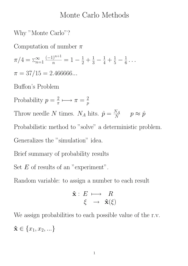
Monte Carlo Methods Why ”Monte Carlo”? Computation of number π ( − 1) n +1 = 1 − 1 2 + 1 3 − 1 4 + 1 5 − 1 � ∞ π/ 4 = 6 . . . n =1 n π = 37 / 15 = 2 . 466666 ... Buffon’s Problem Probability p = 2 → π = 2 π �− p p = N A Throw needle N times. N A hits. ˆ p ≈ ˆ p N Probabilistic method to ”solve” a deterministic problem. Generalizes the ”simulation” idea. Brief summary of probability results Set E of results of an ”experiment”. Random variable: to assign a number to each result x : E �− → R ˆ ξ → x ( ξ ) ˆ We assign probabilities to each possible value of the r.v. x ∈ { x 1 , x 2 , ... } ˆ 1

Value x i with probability p i = P ( ˆ x = x i ): p i ≥ 0 , i p i = 1 � x continuum variable: ˆ � b P ( ˆ x ∈ [ a, b ]) = a f ˆ x ( x ) dx f ˆ x ( x ) : probability density function of the random variable ˆ x . f ˆ x ( x ) ≥ 0 � ∞ −∞ f ˆ x ( x ) dx = 1 Probability distribution function F ˆ x ( x ): � x F ˆ x ( x ) = −∞ f ˆ x ( x ) dx Interpretation: P ( x ≤ ˆ x ≤ x + dx ) = f ˆ x ( x ) dx � P ( ˆ x ∈ Ω) = Ω f ˆ x ( x ) dx P ( ˆ x ≤ x ) = F ˆ x ( x ) P ( x 1 ≤ ˆ x ≤ x 2 ) = F ˆ x ( x 2 ) − F ˆ x ( x 1 ) Discrete case: sum of Dirac-delta functions: f ˆ x ( x ) = ∀ i p i δ ( x − x i ) � 2

Average value of g ( x ): � ∞ � g � ˆ x = E ˆ x [ g ] = −∞ f ˆ x ( x ) g ( x ) dx � g � = ∀ i p i g ( x i ) � x n � n -order moments: � ˆ Mean: µ = � ˆ x � Variance: σ 2 [ ˆ x − µ ) 2 � = � ˆ x 2 � − � ˆ x � 2 . x ] = � ( ˆ σ [ ˆ x ]:root mean square (rms) of the r.v. ˆ x . Bernouilli Distribution : A , ¯ A . x = 0 if results ¯ x = 1 if results A , ˆ A ˆ p ( ˆ x = 0) = p p ( ˆ x = 1) = 1 − p ≡ q � ˆ x � = p σ 2 [ ˆ x ] = p (1 − p ) Binomial Distribution : Repetition of binary experiment N times 3

x i = 1 , 0 ˆ ˆ � N N A = i =1 ˆ x i ˆ N A p = ˆ N � N p ( ˆ p n (1 − p ) N − n � N A = n ) = n � ˆ N A � = Np σ 2 [ ˆ N A ] = Np (1 − p ) � ˆ p � = p p ] = p (1 − p ) σ 2 [ ˆ N Geometric Distribution : To repeat binary experiment un- til one gets A x : number of trials. ˆ x = n ) = (1 − p ) n − 1 p p ( ˆ n = 1 , 2 , . . . , ∞ x � = 1 � ˆ p p 2 − 1 1 σ 2 [ ˆ x ] = p Poisson Distribution : Independent repetition with frequency λ x : number of occurrences per unit time ˆ x = n ) = λ n n ! e − λ p ( ˆ � ˆ x � = λ σ 2 [ ˆ x ] = λ 4

x , ˆ Uniform distribution : continuum r.v. : ˆ U ( a, b ) 1  if x ∈ [ a, b ]  f ˆ x ( x ) =  b − a 0 otherwise   x � = a + b � ˆ 2 x ] = ( b − a ) 2 σ 2 [ ˆ 12 y is ˆ Theorem: ˆ x , F ˆ x ( x ) , let ˆ y = F ˆ x ( ˆ x ) �− → ˆ U (0 , 1). Gaussian Distribution : ˆ G ( µ, σ )  − ( x − µ ) 2 1   √ f ˆ x ( x ) = 2 π exp     2 σ 2 σ  x ( x ) = 1 2 + 1  x − µ   √ F ˆ 2erf    σ 2 5

where erf( z ) is the error function defined as: 2 0 e − y 2 dy � z √ π erf( z ) = Moivre–Laplace Theorem :   N p ( ˆ  p n (1 − p ) N − n N A = n ) =       n  − ( n − Np ) 2 / 2 Np (1 − p ) � � ≈ exp � 2 πNp (1 − p ) � if N → ∞ with | n − Np | / Np (1 − p ) finite. In practice, N ≥ 100 if p = 0 . 5, N ≥ 1000 si p = 0 . 1. 6

√ Poisson λ → ˆ G ( λ, λ ), if λ → ∞ ( λ ≥ 100). 7

Sequence of Random Variables Joint density probability function f ˆ x N ( x 1 , ..., x N ) x 1 ,..., ˆ � P (( ˆ x 1 , ..., ˆ x N ) ∈ Ω) = Ω dx 1 .... dx N f ˆ x N ( x 1 , ..., x N ) x 1 ,..., ˆ x 1 , ... ˆ x N independent r.v. : ˆ f ˆ x N ( x 1 , ..., x N ) = f ˆ x 1 ( x 1 ) . . . f ˆ x N ( x N ) x 1 ,..., ˆ � g ( x 1 , ..., x N ) � = 8

� ∞ � ∞ −∞ dx 1 . . . −∞ dx N g ( x 1 , ...x N ) f ˆ x N ( x 1 , ..., x N ) x 1 ,..., ˆ If ˆ x 1 , ... ˆ x N are independent: � λ 1 g 1 ( x 1 ) + ... + λ N g N ( x N ) � = λ 1 � g 1 ( x 1 ) � + ...λ N � g N ( x N ) � σ 2 [ λ 1 g 1 + ... + λ N g N ] = λ 2 1 σ 2 [ g 1 ] + ... + λ 2 N σ 2 [ g N ] Cros-correlation (covariance) between ˆ x i , ˆ x j : C [ ˆ x i , ˆ x j ] ≡ C ij ≡ � ( ˆ x i − µ i )( ˆ x j − µ j ) � If ˆ x i , ˆ x j are independent: C ij = σ 2 [ ˆ x i ] δ ij Varianza of sum of two functions g 1 ( x ) , g 2 ( x ): σ 2 [ g 1 + g 2 ] = � ( g 1 + g 2 ) 2 � − � g 1 + g 2 � 2 expanding and reordering: σ 2 [ g 1 + g 2 ] = σ 2 [ g 1 ] + σ 2 [ g 2 ] + 2 C [ g 1 , g 2 ] Correlation coefficient ρ [ ˆ x i , ˆ x j ], between ˆ x i , ˆ x j : x j ] = C [ ˆ x i , ˆ x j ] ρ [ ˆ x i , ˆ σ [ ˆ x i ] σ [ x j ] 9

| ρ [ ˆ x i , ˆ x j ] | ≤ 1 Marginal probability density functions: � ∞ f ˆ x 1 ( x 1 ) = −∞ f ˆ x 2 ( x 1 , x 2 ) dx 2 x 1 ˆ � ∞ � ∞ f ˆ x 4 = −∞ dx 1 −∞ dx 3 f ˆ x 4 ( x 1 , x 2 , x 3 , x 4 ) x 2 ˆ x 1 ˆ x 2 ˆ x 3 ˆ Joint Gaussian random variables � � | A |  − 1 �   N � � f ( x 1 , ..., x N ) = (2 π ) N exp i,j =1 ( x i − µ i ) A ij ( x j − µ j ) � �   �  2 � ˆ x i � = µ i C ij = ( A − 1 ) ij Interpretation of the rms. Statistical errors. x ( ξ ) − µ |≤ k σ ) ≥ 1 − 1 P ( | ˆ k 2 Gaussian random variable: x ( ξ ) − µ |≤ k σ ) = erf( k √ P ( | ˆ 2) which takes the following values: P ( | ˆ x ( ξ ) − µ |≤ σ ) = 0 . 68269 ... 10

P ( | ˆ x ( ξ ) − µ |≤ 2 σ ) = 0 . 95450 ... P ( | ˆ x ( ξ ) − µ |≤ 3 σ ) = 0 . 99736 ... µ = ˆ x ( ξ ) ± σ p = ˆ N A /N Buffon’a problem: we measure ˆ Follows the binomial distribution � ˆ p � = p p ] = p (1 − p ) σ 2 [ ˆ N � � � p (1 − p ) p (1 − ˆ p ) � ˆ � � � � p = ˆ p ± � ≈ ˆ p ± � � � N N Error decreases as N − 1 / 2 . p = 2 /π = 0 . 6366, N = 100, relative error ≈ 7 . 5%. We do not know σ . Take the sample mean: µ N = 1 N ˆ i =1 ˆ x i � N � ˆ µ N � = � ˆ x i � = µ Sample variance: 2  1 N  1  1  N N  N  µ N ) 2 = σ 2 x 2 ˆ N = i =1 ( ˆ x i − ˆ i − i =1 ˆ i =1 ˆ x i � � �        N − 1 N − 1 N N  σ 2 N � = σ 2 � ˆ 11

µ N ] = 1 σ 2 [ˆ N σ 2 σ µ N (Ξ) ± ˆ σ N [Ξ] √ √ µ = ˆ µ N (Ξ) ± σ [ˆ µ N ] = ˆ µ N (Ξ) ± N ≈ ˆ N N → ∞ , central limit theorem G ( µ, σ µ N → ˆ √ ˆ N ) Asymptotic result:  σ N (Ξ) − σ |≤ k ˆ σ N (Ξ)  = erf( k  √ √ P  | ˆ 2)     2 N σ N (Ξ) ± ˆ σ N (Ξ) √ σ = ˆ 2 N 12