Modern Database Applications Multimedia Databases Data Warehouses - PDF document

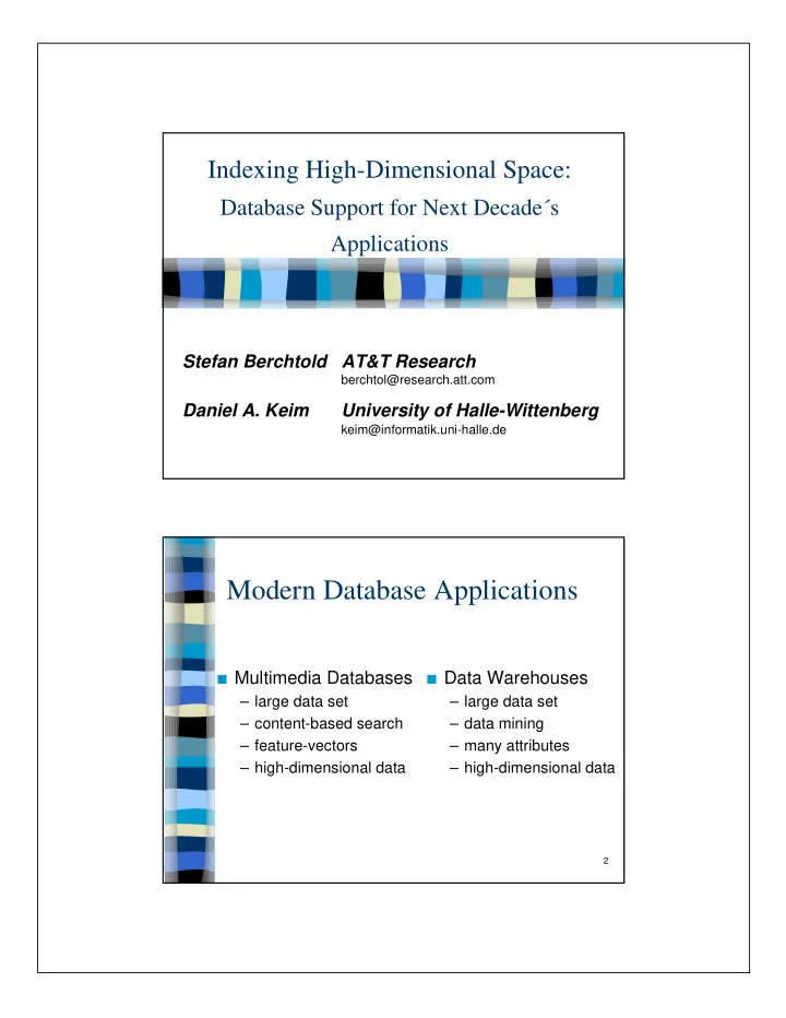
Indexing High-Dimensional Space: Database Support for Next Decade´s Applications Stefan Berchtold AT&T Research berchtol@research.att.com Daniel A. Keim University of Halle-Wittenberg keim@informatik.uni-halle.de Modern Database Applications ■ Multimedia Databases ■ Data Warehouses – large data set – large data set – content-based search – data mining – feature-vectors – many attributes – high-dimensional data – high-dimensional data 2

Overview 1. Modern Database Applications 1. Modern Database Applications 2. Effects in High-Dimensional Space 2. Effects in High-Dimensional Space 3. Models for High-Dimensional Query Processing 3. Models for High-Dimensional Query Processing 4. Indexing High-Dimensional Space 4. Indexing High-Dimensional Space 4.1 kd-Tree-based Techniques 4.2 R-Tree-based Techniques 4.3 Other Techniques 4.4 Optimization and Parallelization 5. Open Research Topics 5. Open Research Topics 6. Summary and Conclusions 6. Summary and Conclusions 3 Effects in High-Dimensional Spaces ■ Exponential dependency of measures on the dimension ■ Boundary effects ■ No geometric imagination � Intuition fails The Curse of Dimensionality The Curse of Dimensionality 4

Assets ■ N data items ■ d dimensions ■ data space [0, 1] d ■ q query (range, partial range, NN) ■ uniform data ■ but not: N exponentially depends on d 5 Exponential Growth of Volume ■ Hyper-cube ( , ) = d Volume edge d edge cube ( , ) Diagonal cube edge d = edge ⋅ d ■ Hyper-sphere π d ( , ) = d ⋅ Volume radius d radius sphere Γ ( / 2 + 1 ) d 6

The Surface is Everything ■ Probability that a point is closer than 0.1 to a ( d -1)-dimensional surface 1 0.9 0.1 0 0.1 0.9 1 7 Number of Surfaces ■ How much k -dimensional surfaces has a d -dimensional hypercube [0..1] d ? 111 *** 010 d   11* ⋅ 2 ( − ) **1   d k   k   001 000 100 8

“Each Circle Touching All Boundaries Includes the Center Point” ■ d -dimensional cube [0, 1] d ■ cp = (0.5, 0.5, ..., 0.5) ■ p = (0.3, 0.3, ..., 0.3) ■ 16- d : circle ( p , 0.7), distance ( p , cp)=0.8 TRUE cp p circle( p, 0.7) 9 Database-Specific Effects ■ Selectivity of queries ■ Shape of data pages ■ Location of data pages 10

Selectivity of Range Queries ■ The selectivity depends on the volume of the query 11 Selectivity of Range Queries ■ In high-dimensional data spaces, there exists a region in the data space which is affected by ANY range query (assuming uniformity) 12

Shape of Data Pages ■ uniformly distributed data � each data page has the same volume ■ split strategy: split always at the 50%-quantile ■ number of split dimensions: ■ extension of a “typical” data page: 0.5 in d’ dimensions, 1.0 in ( d-d’ ) dimensions 13 Location and Shape of Data Pages ■ Data pages have large extensions ■ Most data pages touch the surface of the data space on most sides 14

Models for High-Dimensional Query Processing ■ Traditional NN-Model [FBF 77] ■ Exact NN-Model [BBKK 97] ■ Analytical NN-Model [BBKK 98] ■ Modeling the NN-Problem [BGRS 98] ■ Modeling Range Queries [BBK 98] 15 Traditional NN-Model ■ Friedman, Finkel, Bentley-Model [FBF 77] Assumptions: – number of data points N goes towards infinity ( � unrealistic for real data sets) – no boundary effects ( � large errors for high-dim. data) 16

Exact NN-Model [BBKK 97] ■ Goal: Determination of the number of data pages which have to be accessed on the average ■ Three Steps: 1. Distance to the Nearest Neighbor 2. Mapping to the Minkowski Volume 3. Boundary Effects 17 Exact NN-Model 1. Distance to the Nearest Neighbor 2. Mapping to the Minkowski Volume data space 3. Boundary Effects S • NN data pages • Distribution function ( ) ( ) P NN − dist = r = 1 − P None of the N points intersects NN - sphere N d = ( 1 – ( 1 – Vol avg ( ) r ) ) Density function d d ( ) ( ) ( ) ( ) − 1 N 1 P NN − dist = r = Vol d r ⋅ N ⋅ − Vol d r avg avg 18 dr dr

Exact NN-Model 1. Distance to the Nearest Neighbor 2. Mapping to the Minkowski Volume 3. Boundary Effects 1 1 - a Vol Sp r a 2 ⋅ ⋅ ( ) - - S 2 r a        2 1 - Vol Sp r ⋅ ( ) - - 4 d  d  Minkowski Volume: Vol Mink d r a d – i Vol Sp i r ∑ = ( )   ⋅ ⋅ ( ) i   19 i = 0 Exact NN-Model 1. Distance to the Nearest Neighbor 2. Mapping to the Minkowski Volume 3. Boundary Effects S Generalized Minkowski Volume with boundary effects: N   where d’ log 2 -- -- -- -- - - = C eff   20

Exact NN-Model #S 21 Comparison with Traditional Model and Measured Performance 22

Approximate NN-Model [BBKK 98] 1. Distance to the Nearest-Neighbor Idea: Nearest-neighbor Sphere contains 1/ N of the volume of the data space 1 1 Γ d 2 ( ⁄ + 1 ) d Vol Sp ( ) = - - - - ⇒ NN-dist N d ( , ) = - - - - - - - ⋅ - - - - - - - - - - - - - - - - - - - - - - - - - - - - NN-dist d N N π 23 Approximate NN-Model 2. Distance threshold which requires more data pages to be considered 1 Query Point radius NN-sphere (0.4) NN-sphere (0.6) NN-dist N d = i ( , ) ⋅ 0.5 0 1 Γ d 2 + 1 2 ( ⁄ )  -- -- -- - - -- -- -- -- -- -- -- -- -- -- -- -- -- -  ⋅ d 3 N   π 2 ⋅ d π d ⋅ ⇔ i =  -- -- -- -- -- -- -- -- -- -- -- -- -- -- -- -- -- -- -- -- -- -- -  ⇒ i ≈ -- -- -- -- - - ⋅ -- -- -- -- -- -- - - d e π ⋅ 0.5 4 N 2   ⋅   24

Approximate NN-Model 3. Number of pages π d 3 π d 3 2 d ⋅ ⋅ 2 d ⋅ ⋅ - -- -- -- -- - -- -- -- -- -- -- - - - -- -- - -- - - - -- -- -- -- -- -- - ⋅ ⋅ d d e π e π ⋅ ⋅ 4 N 2 ⋅ 4 N 2 ⋅ N   log 2 - - - - - - - - - d’     ∑ ∑   #S d = = C eff ( )     k   k k = 0 k = 0 25 Approximate NN-Model 26 (depending on the database size and the dimension)

Comparison with Exact NN-Model and Measured Performance Measured Exact Analytical 27 The Problem of Searching the Nearest Neighbor [BGRS 98] ■ Observations: – When increasing the dimensionality, the nearest- neighbor distance grows. – When increasing the dimensionality, the farest- neighbor distance grows. – The nearest-neighbor distance grows FASTER than the farest-neighbor distance. d → ∞ – For , the nearest-neighbor distance equals to the farest-neighbor distance. 28

When Is Nearest Neighbor meaningful? ■ Statistical Model: ■ For the d -dimensional distribution holds: lim (var( p ) / ( p ) 2 ) 0 = D E D d d d → ∞ where D is the distribution of the distance of the query point and a data point and we consider a L p metric. ■ This is true for synthetic distributions such as normal, uniform, zipfian, etc. ■ This is NOT true for clustered data. 29 Modeling Range-Queries [BBK 98] ■ Idea: Use Minkowski-sum to determine the probability that a data page (URC, LLC) is loaded rectangle center query window Minkowski sum 30

Indexing High-Dimensional Space ■ Criterions ■ kd-Tree-based Index Structures ■ R-Tree-based Index Structures ■ Other Techniques ■ Optimization and Parallelization 31 Criterions ■ Structure of the Directory ■ Overlapping vs. Non-overlapping Directory ■ Type of MBR used ■ Static vs. Dynamic ■ Exact vs. Approximate 32

The kd-Tree [Ben 75] ■ Idea: Select a dimension, split according to this dimension and do the same recursively with the two new sub-partitions ■ Problem: The resulting binary tree is not adequate for secondary storage ■ Many proposals how to make it work on disk (e.g., [Rob 81], [Ore 82] [See 91]) 33 kd-Tree - Example 34

The kd-Tree ■ Plus: – fanout constant for arbitrary dimension – fast insertion – no overlap ■ Minus: – depends on the order of insertion (e.g., not robust for sorted data) – dead space covered 35 The kdB-Tree [Rob 81] ■ Idea: – Aggregate kd-Tree nodes into disk pages – Split data pages in case of overflow (B-Tree-like) ■ Problem: – splits are not local – forced splits 36

The LSD h -Tree [Hen 98] ■ Similar to kdB-Tree (forced splits are avoided) ■ Two-level directory: first level in main memory ■ To avoid dead space: only actual data regions are coded 37 The LSD h -Tree ■ Fast insertion ■ Search performance (NN) competitive to X-Tree ■ Still sensitive to pre-sorted data ■ Technique of CADR (Coded Actual Data Regions) is applicable to many index structures 38

The VAMSplit Tree [JW 96] ■ Idea: Split at the point where maximum variance occurs (rather than in the middle) ■ sort data in main memory ■ determine split position and recurse ■ Problems: – data must fit in main memory – benefit of variance-based split is not clear 39 R-Tree: [Gut 84] The Concept of Overlapping Regions directory level 1 directory level 2 data pages exact representation . . . 40