SLIDE 1 Modelling with R A Solution to Two Non-linear Regressions Examples
- 1. The data set in the file rat_data.csv gives the production of insulin in experimental
animals, (rats), in response to a mixture of two drugs. The drug doses are in variables x1 and x1, and the response, in suitable units, is in y. The data set comes originally from a paper by Darby and Ellis (1976), Applied Statistics, 25: 298-299. A non-linear regression model of the following form has been suggested:
y = α+δlog
ǫ ∼ N(0,σ2)
Some experimentation has suggested that suitable starting values could be
α = −17, δ = 10, ρ = 0.05, κ = −0.03
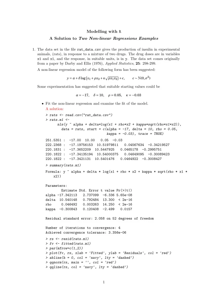
❼ Fit the non-linear regression and examine the fit of the model. A solution: > rats <- read.csv("rat_data.csv") > rats.m1 <- nls(y ~ alpha + delta*log(x1 + rho*x2 + kappa*sqrt(rho*x1*x2)), data = rats, start = c(alpha = -17, delta = 10, rho = 0.05, kappa = -0.03), trace = TRUE) 251.5351 :
10.00 0.05
222.2368 :
10.51979811 0.04567634
220.1831 :
10.5447925 0.0465178
220.1822 :
10.54000375 0.04649095
220.1822 :
10.5401476 0.0464922
> summary(rats.m1) Formula: y ~ alpha + delta * log(x1 + rho * x2 + kappa * sqrt(rho * x1 * x2)) Parameters: Estimate Std. Error t value Pr(>|t|) alpha -17.342113 2.737099
delta 10.540148 0.792484 13.300 < 2e-16 rho 0.046492 0.003263 14.250 < 2e-16 kappa
0.120408
0.0157 Residual standard error: 2.058 on 52 degrees of freedom Number of iterations to convergence: 4 Achieved convergence tolerance: 3.356e-06 > rs <- resid(rats.m1) > fv <- fitted(rats.m1) > par(mfrow=c(1,2)) > plot(fv, rs, xlab = ✬Fitted✬, ylab = ✬Residuals✬, col = ✬red✬) > abline(h = 0, col = ✬navy✬, lty = ✬dashed✬) > qqnorm(rs, main = ✬✬, col = ✬red✬) > qqline(rs, col = ✬navy✬, lty = ✬dashed✬) 1
SLIDE 2
14 16 18 20 22 −4 −2 2 4 Fitted Residuals
−2 −1 1 2 −4 −2 2 4 Theoretical Quantiles Sample Quantiles
These diagnostics give no cause to distrust the model. ❼ Give the parameter estimates and their standard errors. See output above. ❼ Fit the model in the alternative form
y = α+δlog
ǫ ∼ N(0,σ2)
and explain how the parameter estimates are related. A solution would be: > b1 <- coef(rats.m1) > rats.m2 <- nls(y ~ alpha + delta*log(x1 + rho*x2 + kappa*sqrt(x1*x2)), data = rats, start = b1, trace = TRUE) 2627.149 :
10.5401476 0.0464922
384.0291 :
10.30901356 0.04676449
222.4324 :
10.57709815 0.04689004
220.1838 :
10.54367432 0.04654751
220.1822 :
10.54010863 0.04649287
220.1822 :
10.54014612 0.04649222
> summary(rats.m2) Formula: y ~ alpha + delta * log(x1 + rho * x2 + kappa * sqrt(x1 * x2)) Parameters: Estimate Std. Error t value Pr(>|t|) alpha -17.342103 2.737100
delta 10.540146 0.792484 13.300 < 2e-16 rho 0.046492 0.003263 14.250 < 2e-16 kappa
0.025993
0.0158 Residual standard error: 2.058 on 52 degrees of freedom Number of iterations to convergence: 5 Achieved convergence tolerance: 2.851e-06 > b2 <- coef(rats.m2) > c(b2["kappa"], b1["kappa"]*sqrt(b1["rho"])) kappa kappa
2
SLIDE 3 The relationship is, using an obvious notation, κ2 = κ1 ∗ρ1. In the second form the meaning of the κ parameter has changed relative to the first in this way.
- 2. The data set in the file bean_data.csv relates to the growth of an experimental bean
plants. The data originally comes from the book Nonlinear regression modelling: a unified practical approach (1983). Marcel Decker, by David A. Ratkowsky. The variable y gives the length of the plant after a fixed growth time and the variable x the amount of water supplied. Two possible non-linear regression models would be Gompertz :
y = αexp
+ǫ
Logistic :
y = α 1+exp
- −(x−β)/γ
- Self-starting regressin functions are available for both models, namely SSgompertz and
SSlogis in the stats package, (which is attached by default). ❼ Plot the data. ❼ Fit both models and superimpose the fitted lines on the data points in two different colours. A solution to both parts above is as follows: > feijao <- read.csv("bean_data.csv") > with(feijao, plot(x, y, pch=8, cex = 0.7, xlab = "Amount of water", ylab = "Length", ylim = c(0,22))) > pFei <- with(feijao, data.frame(x = seq(min(x), max(x), len = 1000))) > fei.gz <- nls(y ~ SSgompertz(x, alpha, beta, gamma), feijao) > fei.lo <- nls(y ~ SSlogis(x, alpha, beta, gamma), feijao) > pFei.gz <- predict(fei.gz, pFei) > pFei.lo <- predict(fei.lo, pFei) > with(pFei, { lines(x, pFei.gz, col = "navy") lines(x, pFei.lo, col = "red") }) > bstart <- c(delta = 0, coef(fei.gz)) > fei.gz1 <- nls(y ~ delta + alpha*exp(-beta*gamma^x), data = feijao, start = bstart, trace = TRUE) 12.59049 : 0.0000000 22.5065984 8.2175122 0.6783303 10.80006 : 1.7055933 20.2105212 12.1515046 0.6364683 6.978755 : 1.5897493 20.3686624 14.3455543 0.6300065 6.858026 : 1.627120 20.244532 15.696748 0.621974 6.845719 : 1.6431409 20.2193253 16.0527593 0.6204618 6.845284 : 1.6491437 20.2079042 16.1640857 0.6198634 6.845264 : 1.650654 20.205516 16.187592 0.619743 6.845263 : 1.6509895 20.2049639 16.1928599 0.6197152 6.845263 : 1.6510623 20.2048473 16.1939747 0.6197094 6.845263 : 1.6510779 20.2048222 16.1942139 0.6197081 > bstart <- c(delta = 0, coef(fei.lo)) > fei.lo1 <- nls(y ~ delta + alpha/(1 + exp(-(x - beta)/gamma)), data = feijao, start = bstart, trace = TRUE) 3
SLIDE 4
6.210243 : 0.000000 21.508903 6.360354 1.607239 5.20133 : 0.9519087 20.3240469 6.5150838 1.4303138 5.189891 : 0.8844376 20.3987972 6.5012742 1.4332526 5.189891 : 0.8844725 20.3988558 6.5013730 1.4332403 > pFei.gz1 <- predict(fei.gz1, pFei) > pFei.lo1 <- predict(fei.lo1, pFei) > with(pFei, { lines(x, pFei.gz1, col = "navy", lty = "dashed") lines(x, pFei.lo1, col = "red", lty = "dashed") }) > legend("bottomright", c("Observations", "Gompertz", "Logistic", "delta + Gompertz", "delta + Logistic"), pch = c(8, rep(NA, 4)), lty = c(NA, rep(c("solid", "dashed"), each = 2)), col = c("black", rep(c("navy", "red"), 2)), bty = "n", cex = 0.7)
2 4 6 8 10 12 14 5 10 15 20 Amount of water Length
Observations Gompertz Logistic delta + Gompertz delta + Logistic
❼ Extend both models by adding a constant to the model function, say δ. Done above. ❼ In each case, test the model that the additional constant improves the fit. A solution is as follows: > anova(fei.gz, fei.gz1) Analysis of Variance Table Model 1: y ~ SSgompertz(x, alpha, beta, gamma) Model 2: y ~ delta + alpha * exp(-beta * gamma^x) 4
SLIDE 5
Res.Df Res.Sum Sq Df Sum Sq F value Pr(>F) 1 12 12.5905 2 11 6.8453 1 5.7452 9.2323 0.01128 > anova(fei.lo, fei.lo1) Analysis of Variance Table Model 1: y ~ SSlogis(x, alpha, beta, gamma) Model 2: y ~ delta + alpha/(1 + exp(-(x - beta)/gamma)) Res.Df Res.Sum Sq Df Sum Sq F value Pr(>F) 1 12 6.2102 2 11 5.1899 1 1.0204 2.1626 0.1694 In the case of the Gompertz growth model, the fit is significantly improve, but not for the Logistic growt model. ❼ Add the two lines from the extended models to the plot, using the same colors as before, but a different line type. Done above. ❼ Add a legend to your plot stating what the lines and symbols mean. Place the legend in the lower right-hand corner of the plot. Done above. 5