SLIDE 1 Model theory in positive and continuous logics
Itay Ben-Yaacov Logic Colloquium 2005 Athens, Greece July 2005
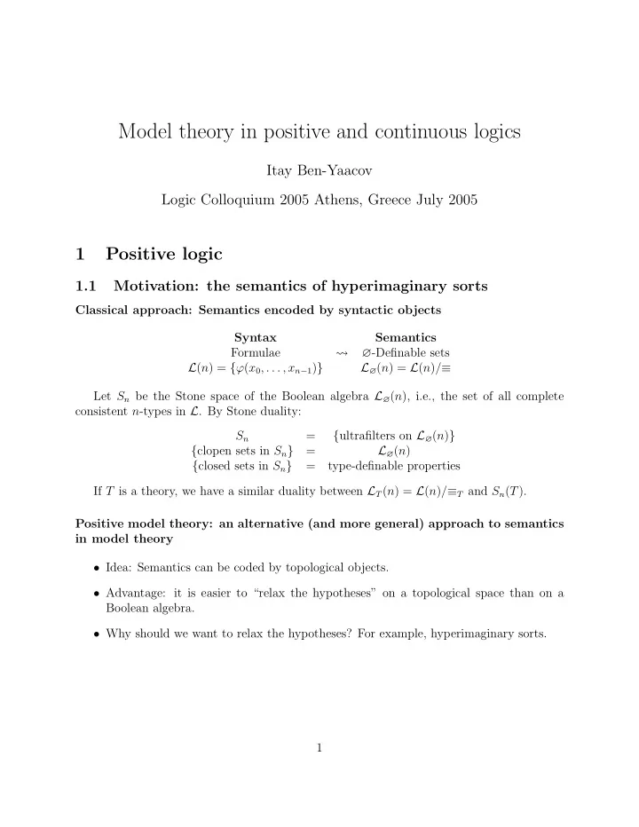
1 Positive logic
1.1 Motivation: the semantics of hyperimaginary sorts
Classical approach: Semantics encoded by syntactic objects Syntax Semantics Formulae
L(n) = {ϕ(x0, . . . , xn−1)} L∅(n) = L(n)/≡ Let Sn be the Stone space of the Boolean algebra L∅(n), i.e., the set of all complete consistent n-types in L. By Stone duality: Sn = {ultrafilters on L∅(n)} {clopen sets in Sn} = L∅(n) {closed sets in Sn} = type-definable properties If T is a theory, we have a similar duality between LT(n) = L(n)/≡T and Sn(T). Positive model theory: an alternative (and more general) approach to semantics in model theory
- Idea: Semantics can be coded by topological objects.
- Advantage: it is easier to “relax the hypotheses” on a topological space than on a
Boolean algebra.
- Why should we want to relax the hypotheses? For example, hyperimaginary sorts.
1
SLIDE 2 Imaginary elements: first order syntax works Let E(¯ x, ¯ y) be a definable equivalence relation on n-tuples, and: L∗ = L ∪ {πE} M ∗ = M ∪ M n/E, πM∗
E (¯
a) = ¯ a/E. T ∗ = ThL∗{M ∗ : M T} = T ∪ {“for all ¯ x, πE(¯ x) is the E-class of ¯ x”}. If M is a monster model of T then M ∗ is a monster model of T ∗; if T is model complete so is T ∗; etc. Example: cosets Let M = G, 1, ·, . . . be a group, and H ≤ G a definable subgroup. Let E(x, y) be the formula ∃z (z ∈ H ∧ x = yz). Then E is a definable equivalence relation, and the sort ME is the sort of left cosets of H: {gH : g ∈ G}. If H is a normal subgroup, then we can define multiplication on ME by the formula ϕ(xE, yE, zE): ∃xy
- πE(x) = xE ∧ πE(y) = yE ∧ πE(xy) = zE
- .
Hypermaginary elements: first order syntax fails Let E(¯ x, ¯ y) be a type-definable equivalence relation on α-tuples (possibly infinite). E-classes are called hyperimaginary elements. If α = n < ω, we may again try to define: L∗ = L ∪ {πE} M ∗ = M ∪ M n/E, πM∗
E (¯
a) = ¯ a/E. T ∗ = ThL∗{M ∗ : M T}. However, even if M is saturated M ∗ needs not be, and in a saturated model N ∗ T ∗ we may find ¯ a, ¯ b such that E(¯ a,¯ b) but πE(¯ a) = πE(¯ b). For the purpose of studying E-classes, T ∗ is useless. 2
SLIDE 3 Example: infinitesimals Let RCF be the theory of real closed fields in the language of ordered rings. Let E(x, y) be “x − y is infinitesimal”. This is type-definable: E(x, y) = {−1/n < x − y < 1/n: n < ω}. If M RCF then the set πE(x) = πE(y) ∪ E(x, y) is finitely realised in M ∗, but not
- realised. It would be realised in a saturated model of T ∗, which means that πE is not what
we want it to be. Solution: semantics via types Let U be a monster model for T, UE = U α/E a hyperimaginary sort. As sets: Sn(T) = U n/ Aut(U), Sα(T) = U α/ Aut(U), etc.
We obtain a projection Sα(T) ։ SE(U). We equip SE(U) with the quotient topology: it is compact and Hausdorff. We can similary construct Sn,m×E(T) (n real elements, m E-classes), and do the same with more than one equivalence relation. From definable sets to type-definable ones We have a new feature: the type-space SE(T) is not necessarily totally disconnected (no base of clopen sets). Hence, no Stone duality with a Boolean algebra, and no canonical notion of a for- mula/definable set. We do have a formal analogue of the notion of type-definable properties, i.e., properties definable by a set of formulae, through the classical correspondence: type-definable properties ↔ closed sets of types. The family of type-definable properties is closed under conjunction, disjunction, existen- tial (and universal) quantification, but not negation. It also satisfies: Compactness for type-definable properties If {pi(¯ x): i ∈ I} is a family of type-definable properties which is finitely satisfiable, then it is satisfiable. Recovering some syntax Let LE consist of a n-ary predicate symbol PR for every closed set R ⊆ Sm×E(T). Let ∆E be the set of all quantifier-free positive LE-formulae. Then UE is naturally an LE structure. The type of a tuple in UE is determined by the ∆E-formulae it satisfies (its ∆E-type), and every finitely satisfiable small set of ∆E-formulae is satisfied (more precise definitions follow). (We can do the same with several sorts simultaneously.) This is our motivating example for positive logic. 3
SLIDE 4 1.2 Positive fragments and universal domains
Syntax for positive logic Let L be any first order language.
- Definition. A positive fragment of L is a subset ∆ ⊆ L closed under positive Boolean
combinations, change of variables and sub-formulae. (Caution: only ∧,∨,¬,∃ are allowed.) We fix a positive fragment ∆ and define: Σ = ∃∆ = {∃¯ y ϕ(¯ x, ¯ y): ϕ ∈ ∆} (positive existential formulae) Π = ¬Σ = {∀¯ y ¬ϕ(¯ x, ¯ y): ϕ ∈ ∆} (negative universal formulae) Note that Σ is also a positive fragment. Universal domains
- Definition. A (partial) ∆-homomorphism between two structures f : M → N (f : M
N) is a mapping such that for all ¯ a ∈ dom(f) and ϕ(¯ x) ∈ ∆: M ϕ(¯ a) = ⇒ N ϕ(f(¯ a)).
- Definition. A (κ-)universal domain is an L-structure U satisfying:
- ∆-Compactness: Every small (< κ) set of ∆-formulae which is finitely realised in U is
realised in U.
- ∆-Homogeneity: Every partial ∆-homomorphism f : U U with small domain ex-
tends to an automorphism of U.
- Elimination of ∃: Every Σ-formula ∃¯
y ϕ(¯ x, ¯ y) is equivalent in U to some partial ∆-type p(¯ x). Complete positive Robinson theories Universal domains replace the monster models: big homogeneous models in which the saturation assumption is restricted to our positive fragment ∆. Therefore: A partial ∆-type (i.e., a set of ∆-formulae) Φ(¯ x) is realised in U if and only if it is consistent with its negative universal theory: T = ThΠ(U) = {∀¯ x ¬ϕ(¯ x): ϕ ∈ ∆ and U ∀¯ x ¬ϕ(¯ x)}. We therefore say that U is a universal domain for T.
- Definition. A complete positive Robinson theory is a Π-theory which has a universal domain.
4
SLIDE 5 Examples
- Example. If ∆ = Lω,ω, T is a complete first order theory, and U is a monster model of T.
We call this the “first order” case.
- Example. With UE and ∆E as constructed in the example of hyperimaginaries, UE is a
universal domain with respect to ∆E.
- Example. If ∆ is closed for negation, T is a Robinson theory and U is its universal domain
(Hrushovski [Hru97]), whence the term “positive Robinson theory”.
1.3 On ∆-inductive theories and e.c. models
∆-inductive limits Fix a positive fragment ∆ of L. Here ∆-homomorphisms will play the role of embeddings. Note that a ∆-homomorphism f : M → N needs not be injective, so we cannot say that N extends M. Instead, we will say that N continues M. ∆-inductive limits Let (I, <) be totally ordered, (Mi : i ∈ I) be structures, and for each i < j let fij : Mi → Mj be a ∆-homomorphism such that fjk ◦ fij = fik. One can construct in the obvious manner a direct limit N = lim − → Mi, equipped with ∆-homomorphisms gi : Mi → M, such that gj ◦ fij = gi for i < j. If ∆ = {q.f. formulae}. . . Then a ∆-homomorphism is an embedding, and a ∆-inductive limit is an increasing union. ∆-inductive theories
- Definition. A first order theory T is ∆-inductive if an inductive limit of models of T is a
model of T. For example, every Π-theory is ∆-inductive. More generally: Lemma (Characterisation of ∆-inductive theories). A first order theory T is ∆- inductive if and only if it can be axiomatised by sentences of the form ∀¯ x∃¯ y ϕ(¯ x) → ψ(¯ x, ¯ y) ϕ, ψ ∈ ∆. If ∆ = {q.f. formulae}. . . This is the classical characterisation of inductive theories. 5
SLIDE 6 Existentially closed (e.c.) models
- Definition. A model M of a theory T is existentially closed if for every ∆-homomorphism
f : M → N T, and every ¯ a ∈ M and ϕ(¯ x, ¯ y) ∈ ∆: N ∃¯ y ϕ(f(¯ a), ¯ y) = ⇒ M ∃¯ y ϕ(¯ a, ¯ y). We can use the classical chain argument to show: Lemma (Existence of existentially closed models). If T is ∆-inductive and M T, then M continues to an e.c. model N T. (Uses the Axiom of Choice.) If ∆ = {q.f. formulae}. . . This is the classical definition of e.c. models. Companions We will be interested in what happens in the class of e.c. models of a ∆-inductive theory. If two such theories have precisely the same e.c. models, we call them companions, and for
- ur purposes they are equivalent.
- Lemma. The companionship class of a ∆-inductive theory T is determined by the set of
Π-consequences of T, denoted TΠ. Therefore, on the one hand we may restrict our consideration to Π-theories. On the
- ther, when it is convenient to consider other ∆-inductive theories, we are allowed to do so.
Example (Positive Morleyisation). Let ∆ ⊆ Lω,ω be a positive fragment, and T an ∆- inductive theory (e.g., a Π-theory). L′ = {Rϕ(¯ x): ϕ(¯ x) ∈ ∆} ∆′ = positive quantifier-free L′-formulae T ′ = ∀¯ x∃¯ y Rϕ(¯ x) → Rψ(¯ x, ¯ y) ∀¯ x∃¯ y ϕ(¯ x) → ψ(¯ x, ¯ y) ∈ T ∀¯ x∃!y Rf(¯
x)=y(¯
x, y) f ∈ L ∀¯ x R¬ϕ(¯ x) ↔ ¬Rϕ(x) ¬ϕ ∈ ∆ ∀¯ x R∃¯
yϕ(¯
x) ↔ ∃¯ y Rϕ(¯ x, ¯ y) ∃¯ yϕ ∈ ∆ . . . (same for ∨, ∧) Then T ′ is ∆′-inductive, and up to a change of language it has the same e.c. models as T. ∴ We may always assume that ∆ consists only of positive quantifier-free formulae. 6
SLIDE 7 Positive Robinson theories, revisited We can now re-define positive Robinson theories by a “quantifier elimination” property:
- Definition. Let T be a ∆-inductive theory. It is:
- A positive Robinson theory if every Σ-formula ∃¯
y ϕ(¯ x, ¯ y) is equivalent, in the class of e.c. models of T, to a partial ∆-type (a set of ∆-formulae).
- Complete if every two models of T continue to a third (“positive JEP”).
Our new definition of a complete positive Robinson theory agrees with the previous one:
- Theorem. A Π-theory is a complete positive Robinson theory if and only if it has a κ-
universal domain for some (all) big enough κ.
⇒: The class of e.c. models of T has enough amalgamation properties to construct a sufficiently homogeneous e.c. model of T in which all small e.c. models ∆-embed. ⇐ =: Verify the definition for small (cardinality < κ) e.c. models by ∆-embedding them in the universal domain. The same properties for arbitrary e.c. models follow easily. Types and type spaces
- Classical concepts and methods transfer (mostly) to positive logic:
Monster model Universal domain
∆
- Types (over a small set A ⊆ U):
tp(¯ a/A) = {ϕ(¯ x,¯ b): ϕ ∈ ∆,¯ b ∈ A, U ϕ(¯ a,¯ b)} Sn(A) = U n/ AutA(U) = {tp(¯ a/A): ¯ a ∈ U n}
- Topology: every ∆-formula with parameters in A defines a closed subset:
[ϕ(¯ x, ¯ a)] = {p(¯ x) ∈ Sn(A): ϕ(¯ x, ¯ a) ∈ p}. These sets form a base of closed sets for a compact, T1 topology. A word of caution Because there is no canonical notion of a formula, the choice of language is even more arbitrary than in first order logic: ∆-formulae define closed sets of types (i.e., a partial type), but a closed set of types may or not be defined by a ∆-formula. If such a closed set is not definable by a ∆-formula, we can always expand the language so that it is. The semantic contents, coded by the type spaces, would not change. Therefore: Different positive Robinson theories in different (arbitrary!) languages with the homeomor- phic type spaces are to be considered equivalent. The common semantic contents will be referred to as a compact abstract theory, or cat. 7
SLIDE 8 1.4 Simplicity
Closing the circle: simplicity Our motivation for positive logic was the notion of hyperimaginary elements. These were introduced by Hart, Kim and Pillay [HKP00] for the construction of canonical bases in first
They had to re-prove for hyperimaginaries most of the theorems concerning independence in simple theories. One can define indiscernible sequences, non-dividing and simplicity (= local character of non-dividing) in the positive setting. Caution: not all equivalent definitions of first order logic are equivalent.) Definition.
ai : i < ω) is indiscernible over A if for all i0 < i1 < . . . < in−1 < ω: tp(¯ ai0, . . . , ¯ ain−1/A) depends solely on n.
x,¯ b, A) ∈ Sn(¯ bA) divides over A if There exists an A-indiscernible sequence (¯ bi : i < ω) such that ¯ b0 = ¯ b, and
i<ω p(¯
x,¯ bi, A) is inconsistent.
a/¯ bC) does not divide over C for all ¯ a ∈ A, ¯ b ∈ B, we say that A and B are independent over C, in symbols A | ⌣C B.
- A cat T is simple if for all a and A there is A0 ⊆ A, |A0| ≤ |L|, such that a |
⌣A0 A.
- Theorem. If T is simple, then |
⌣ satisfies:
⌣C B ⇐ ⇒ B | ⌣C A.
⌣B CD ⇐ ⇒
⌣B C ∧ A | ⌣BC D
- .
- Invariance, finite character, local character.
- Extension only holds for some types (e.g., types over sufficiently saturated models). We
call such types extendible.
- Independence theorem for extendible Lascar strong types.
Conversely, if |′ ⌣ satisfies these hypotheses, then T is simple and |′ ⌣ = | ⌣. Moreover, extendible Lascar strong types admit hyperimaginary canonical bases. As we may add hyperimaginary sorts and remain within positive logic, we may always assume that canonical bases exist in the structure, achieving our original goal.
- Definition. A cat T is Hausdorff if Sn(T) is Hausdorff for all n. It follows that Sα(A) is
Hausdorff for every α and set of parameters A.
- Example. Adding hyperimaginary sorts to a first order theory (as in the beginning) yields a
Hausdorff cat. 8
SLIDE 9
- Theorem. If T is Hausdorff (in fact, a weaker assumption, “thickness”, suffices) then:
- Every type has non-dividing extensions to arbitrary sets.
- The theory of hyperdefinable groups [Wag01] holds.
- Lovely/beautiful pairs construction can be carried out.
- Etc.
2 Continuous first order logic
2.1 Characterising first order logic
Going back a bit closer to first order logic
- It really is fun to look for the most general context in which a certain argument works.
- But our original goal was merely to “relax the conditions defining first order logic”,
whatever that means. So what precisely does define the full first order logic? Let T be a complete first order theory (equivalently: a positive Robinson theory with ∆ = Lω,ω). Then:
- Sn(T) is totally disconnected for all T (i.e., has a base of clopen sets).
- The restriction mapping Sn+1(T) → Sn(T) is open.
If a cat satisfies the latter property we say it is open. (The mapping Sn+1(T) → Sn(T) is continuous and closed for every cat.) Conversely, let T be a cat:
- If Sn(T) is totally disconnected for all n, then we may choose a language for it such
that ∆ is closed for negation.
- Then, T being open is equivalent to the class of e.c. models of T being elementary, or
to any universal domain being a saturated model of its own theory. 9
SLIDE 10 First order logic without negation?!
- When adding a hyperimaginary sort we relaxed the first condition, replacing “totally
disconnected” with “Hausdorff” (which is indeed next-best.)
- In the totally disconnected case (i.e., “with negation”), openness of Sn+1(T) → Sn(T)
meant the existence of a first order model completion for T. In the case without negation, does it still mean that some kind of a first order model completion exists?
- Surprisingly enough: YES.
- By the way, hyperimaginary sorts do satisfy the openness hypothesis.
- Convention. From now on we assume T is an open Hausdorff cat, i.e., that Sn(T) is
Hausdorff and Sn+1(T) → Sn(T) is open for all n. Continuous predicates
- A compact totally disconnected topology is given by the family of clopen sets; equiva-
lently: by the family of functions to {0, 1} (also known as {T, F}).
- Similarly: A compact Hausdorff topology is given by the family of all continuous
functions to [0, 1] (or to C).
- In first order logic, a continuous mapping from Sn(T) to {0, 1} is simply a formula, or
a definable n-ary predicate.
- By analogy, we define:
- Definition. A (definable) continuous n-ary predicate is a continuous mapping ϕ: Sn(T) →
[0, 1]. For a tuple ¯ a ∈ U n we write ϕ(¯ a) instead of ϕ(tp(¯ a)). A lemma concerning open mappings
- Lemma. Let X and Y be compact Hausdorff space, f : X ։ Y a continuous (=
⇒ closed) and open projection. Let ϕ: X → [0, 1] be a continuous mapping, and define ψ(y) = inf
x∈f−1(y) ϕ(x).
Then ψ: Y → [0, 1] is continuous.
- Proof. For any r ∈ [0, 1]: ψ−1([0, r]) = f(ϕ−1([0, r])) is closed.
Assume now that ψ(y) < r: then there is x ∈ f −1(y) such that ϕ(x) < r, and there is a neighbourhood U of x such that ϕ(U) ⊆ [0, r). Then f(U) is a neighbourhood of y, and ψ(f(U)) ⊆ [0, r). Thus ψ−1([0, r)) is
10
SLIDE 11 Operations on continuous predicates
- Variable manipulation: If ϕ(x, y) is a definable predicate, then so are:
ψ(x, y, z) := ϕ(x, y) (dummy variables) χ(x) := ϕ(x, x) (repetition of variables).
- Continuous (instead of Boolean) combinations: If f : [0, 1]2 → [0, 1] is continuous
and ϕ(x, y) and ψ(x, z) are definable continuous then so is: χ(x, y, z) := f(ϕ(x, y), ψ(x, z)).
- Continuous quantification: If ϕ(¯
x, y) is a definable continuous predicate, then so are: ψ(¯ x) := inf
y ϕ(¯
x, y) χ(¯ x) := sup
y ϕ(¯
x, y). (Applying the Lemma to Sn+1(T) → Sn(T).) An (important) example Assume |L| ≤ ω. As [x = y] ⊆ S2(T) is closed, it is the zero set of a continuous mapping ϕ: S2(T) → [0, 1]. In other words, we have a definable continuous predicate ϕ(x, y) such that for every a, b ∈ U: ϕ(a, b) = 0 ⇐ ⇒ a = b. Let d(x, y) := supz |ϕ(x, z) − ϕ(y, z)|. Then d is also a definable continuous predicate, satisfying: d(x, y) = d(y, x) d(x, y) ≤ d(x, w) + d(w, x) d(x, y) = 0 ⇐ ⇒ x = y. In other words, d is a definable metric. Uniform continuity
x) is an n-ary definable continuous predicate, let [ϕ(¯ x) ≤ r] denote the (closed) set {p ∈ Sn(T): ϕ(p) ≤ r}. Let ϕ(x, ¯ z) be any definable continuous predicate, and ε > 0. Then: [sup
¯ z |ϕ(x, ¯
z) − ϕ(y, ¯ z)| ≥ ε] ∩
[d(x, y) ≤ δ] = ∅. 11
SLIDE 12 By compactness, there is δ > 0 such that for all a, b ∈ U: d(a, b) ≤ δ = ⇒ sup
¯ z |ϕ(a, ¯
c) − ϕ(b, ¯ c)| < ε. In other words, every definable continuous predicate is uniformly continuous with respect to d. A similar argument shows that if f : U n → U is type-definable (i.e., its graph is) then it is uniformly continuous. If d′ is another definable metric, then d and d′ are uniformly continuous w.r.t. each other, i.e., they are uniformly equivalent. We have all we need to motivate continuous logic. (Another motivation: local stability. Not in this talk.)
2.2 Formal definitions
Continuous logic Continuous first order logic as presented here was defined independently by B. and Usvy- atsov [BUa]. It is similar to the logic defined by Chang & Keisler [CK66], but is far better adapted to our needs.
- We replace the set of truth values {T, F} with the compact interval [0, 1]. (It turns
- ut to be more elegant to identify “True” with 0 rather than 1.)
- The distinguished equality symbol = is replaced with a distinguished metric symbol d.
- First order logic requires that = be a congruence relation for all predicate and function
- symbols. Analogously, we require that all symbols be uniformly continuous w.r.t. d.
- Definition. A continuous signature is a collection L of predicate and function symbols,
with various arities, where each symbol s is equipped with a uniform continuity modulus ε → δs(ε). Continuous structures
- Definition. A continuous pre-L-structure consists of:
- A set M0.
- For each n-ary predicate symbol a mapping P M0 : M n
0 → [0, 1].
- For each n-ary function symbol a mapping f M0 : M n
0 → M0.
Such that in addition dM0 is a pseudometric, and all the interpretations of the symbols respect their uniform continuity moduli.
- Definition. A continuous structure is a pre-structure M in which dM is a complete metric.
For every pre-structure M0 we may construct its completion M = ˆ M0 by modding out d(a, b) = 0 and completing. 12
SLIDE 13 Continuous syntax
- Terms: constructed using variables and function symbols as usual.
- Atomic formulae: defined as usual.
- Connectives: In theory any continuous function f : [0, 1]n → [0, 1]: if ϕi, i < n are
formulae then so is f(ϕ0, . . . , ϕn−1).
- Quantifiers: inf and sup:
sup
x ϕ
inf
x ϕ.
Continuous semantics Writing ϕ(¯ x) we mean that all free variables of ϕ are in ¯ x. If M is a structure, then every term t(¯ x) and formula ϕ(¯ x) induce uniformly continuous mappings (by induction on the structure of the term or formula): tM : M |¯
x| → M
ϕM : M |¯
x| → [0, 1].
For example, if ψ(¯ x) = supy ϕ(¯ x, y), then: ψM(¯ a) = sup{ϕM(¯ a, b): b ∈ M}. A little more about connectives The family of all possible continuous connectives is of the size of the continuum. In practise, it suffices to use: ¬x = 1 − x (unary – like negation) 1 2x = x 2 (unary – no analogue) x − · y =
x ≥ y x < y (binary – like “y → x”) We can get most of the connectives we’d like to use by composing these: |x − y| = ¬(¬(x − · y) − · (y − · x)) By lattice Stone-Weierstrass: every continuous function can be uniformly approximated by terms in ¬, 1
2, −
· . 13
SLIDE 14 2.3 Theories
Statements and compactness
- Definition. A statement is something of the form “r ≤ ϕ(¯
x) ≤ s”. It is closed if ϕ has no free variables. Theorem ( Lo´ s’s Theorem for continuous logic). Let (Mi : i ∈ I) be L-structures, U an ultrafilter on I. Let M = Mi/U . Then for every formula ϕ(¯ x), and tuples ¯ ai ∈ Mi: ϕM([¯ ai : i ∈ I]) = lim
U ϕMi(¯
ai). Corollary (Compactness for continuous first order logic). A set of statements which is finitely satisfiable is satisfiable. Theories
- Definition. A theory is a set of closed statements. (We could restrict to statements of the
form ϕ = 0, so theories are “ideals” – this boils down to the same thing).
- Definition. We say that T eliminates quantifiers if for every formula ϕ(¯
x) and ε > 0 there is a quantifier-free formula θ(¯ x) such that: T sup
¯ x |ϕ − θ| ≤ ε
i.e.: M T = ⇒ (sup
¯ x |ϕ − θ|)M ≤ ε.
Example: probability algebras The language: functional language of Boolean algebras + one unary predicate symbol µ: LPrAlg = {0, 1, ∨, ∧, ·c, µ}. The theory TPrAlg: “Boolean algebra with an additive probability measure; distance is the measure f the symmetric difference”. supx,y d(xc ∧ yc, (x ∨ y)c) = 0 (i.e., ∀xy xc ∧ yc = (x ∨ y)c) . . . axioms of Boolean algebras . . . µ(1) = 1 µ(0) = 0 ∀xy µ(x) + µ(y) = µ(x ∨ y) + µ(x ∧ y) (sup | . . . − . . . | = 0) ∀xy d(x, y) = µ((x ∧ yc) ∨ (y ∧ xc)) TAtlsPrAlg = TPrAlg + “no atoms”: supx infy
2µ(x)
The theory TAtlsPrAlg is complete and eliminates quantifiers (a back-and-forth argument). It the “model completion” of the “universal theory” TPrAlg (note that M ⊆ N TPrAlg = ⇒ M TPrAlg). 14
SLIDE 15 Types
- A complete n-type is a maximal (finitely) satisfiable set p(¯
x) of statements of the form ϕ(¯ x) = rp,ϕ ∈ [0, 1]. We may also view it as a mapping ϕ(¯ x) → ϕ(¯ x)p = rp,ϕ.
a ∈ M is given by: tpM(¯ a) = {ϕ(¯ x) = value of ϕM(¯ a): ϕ(¯ x) ∈ L}.
- The space of all n-types consistent with a theory T is denoted Sn(T). It is equipped
with the minimal topology in which the sets: [r ≤ ϕ(¯ x) ≤ s] := {p: r ≤ ϕp ≤ s} are closed (equivalently: such that all the mappings p → ϕp are continuous).
- T eliminates quantifiers if and only if every p ∈ Sn(T) is determined by the mappings
ϕ → ϕp for quantifier-free ϕ. Back to the motivation The expressive power of an open Hausdorff cat T is the same as that of a continuous first
- rder theory T ′:
- To get from T to T ′: define a continuous language
L′ = {Pϕ n-ary predicate: continuous ϕ: Sn(T) → [0, 1]} T ′ = ThL′(U ′) viewing U as an L′-structure U ′. Then T ′ eliminates quantifiers and U is a monster model.
- To go back, using a monster model U ′ T:
L = {PR n-ary predicate: closed R ⊆ Sn(T ′)} ∆ = {quantifier-free positive formulae} T = ThΠ(U) viewing U ′ as an L′-structure U. Then U is a universal domain for T.
- Going in either direction we have
Sn(T) ∼ = Sn(T ′). 15
SLIDE 16 3 The metric
3.1 In continuous logic, every space is metric. . .
What now? We can proceed to look at:
- Existentially closed models, inductive theories, model completions, model compan-
- ions. . .
- Definability: Beth, Svenonius.
- Saturation, homogeneity. Monster models.
- Omitting types, isolated (and semi-isolated) types, Ryll-Nardzewski.
- Stability, and local stability (counting types ⇐
⇒ non order property ⇐ ⇒ notion of independence).
Many of these require us to take into account the metric on the universal domain, and metrics it induces on other spaces. My message for the day: do not forget the metric In continuous logic, each time we have an object we might think of as a “set with additional structure”, it is in fact a metric space with additional structure (in classical logic the metric is discrete, so these ARE just sets. . . ):
- In a continuous structure, the interpretations of the symbols are uniformly continuous:
this is a (complete) metric space with additional structure.
- Spaces of types admit a natural metric:
d(p, q) = inf{d(¯ a,¯ b): ¯ a p,¯ b q}. (Here d(¯ a,¯ b) = maxi<n d(ai, bi).) Although this may be less obvious, one should view type spaces as metric spaces (rather than sets) with a topological structure: shows up when considering superstability, omitting types, and even ω-saturation. And yet another metric (to be looked at. . . ) If M is a countable discrete structure, then Aut(M) is a polish group in the pointwise convergence topology. The uniform convergence metric is discrete. In the separable metric case, the topological structure of pointwise convergence comes on top of the (non-trivial) metric structure of uniform convergence: 16
SLIDE 17 M is discrete Hilbert space: U(H) Pointwise (polish): . . . Strong operator topology Uniform (metric): discrete Operator norm.
- Question. Can we simply take a categorical definition of a topological space in the category
- f sets, and transfer it to the category of metric spaces?
3.2 Omitting types
“Any fool can realise a type, but it takes a model-theorist to omit one.” G.S. Theorem (Omitting Types Theorem, classical version). Let T be a first order theory in a countable language, and for each n < ω, let Xn ⊆ Sn(T) be meagre. Then there is a model M T omitting every type in Xn.
- Proof. The set of all p ∈ Sω(T) which are types of enumerations of models of T is co-meagre
(Tarski-Vaught test). Removing countably many meagre sets we still have something co- meagre, and in particular non-empty.
- Corollary. A closed set X ⊆ Sn(T) is realised in every model if and only if it has non-empty
interior.
- Theorem. Let T be a continuous first order theory in a countable language, and for each
n < ω, let Xn ⊆ Sn(T) be meagre. Then there is a pre-model M0 T (i.e., a dense subset
- f a model M T) omitting every type in Xn.
Proof: same. The set of all p ∈ Sω(T) which are types of enumerations of pre-models of T is co-meagre (Tarski-Vaught test). . .
- Corollary. A closed set X ⊆ Sn(T) is realised in every dense subset of model if and only if
it has non-empty interior. So what?! Well, we forgot the metric A “classical” example: Isolated (principal) types Recall: d(p, q) = inf{d(¯ a,¯ b): ¯ a p,¯ b q}. The metric limits the resolution: we cannot “see” single points, only balls of positive radius:
- Definition. A type p ∈ Sn(T) is isolated if for every ε > 0, the ε-ball pε is a neighbourhood
- f p.
Theorem (Henson). A type can be omitted in a model if and only if it is non-isolated.
- Proof. If p is not isolated, it’s that pε is nowhere dense for some ε > 0. Then there is a
pre-model M0 which omits pε, and the model M = ˆ M0 omits p. Conversely: construct a convergent sequence. . . 17
SLIDE 18 Omitting more than a single type: 0+-interior Definition.
- Let X ⊆ Sn(T), ε > 0 The ε-interior of X, denoted Xε,◦, is the interior
- f Xε = {p: d(p, X) ≤ ε} (if X is closed, so is Xε).
- The 0+-interior of X is defined as:
X0+,◦ =
Xε,◦.
- X is nowhere 0+-dense if ¯
X0+,◦ = ∅.
- X is 0+-meagre if it is a countable union of nowhere 0+-dense sets.
Real Omitting Types Theorem
- Remark. A type p is isolated if and only if {p}0+,◦ = ∅, if and only {p}0+,◦ = {p}.
Therefore, the omission of non-principal types is a special case of:
- Theorem. Let T be a continuous theory in a countable language.
Let Xn ⊆ Sn(T) be 0+-meagre for all n. Then there exists a model M T omitting Xn.
- Proof. We may assume we only need to omit one X ⊆ Sn(T), that X is closed and X0+,◦ = ∅.
For m < ω define Ym = ∂(X
1 m) = X 1 m X 1 m,◦.
Each Ym is closed and nowhere dense, so there is a pre-model M0 omitting them all. Assume that p ∈ X. Then there is ε > 0 such that p / ∈ X2ε,◦. Let W = Xε,◦. Then W is open, and it follows that W <ε is also open, so W <ε ⊆ X2ε,◦. Therefore d(p, W) ≥ ε. Let m > 1
ε. Then p
1 m ⊆ X 1 m, and
p
1 m ∩ X 1 m,◦ ⊆ p<ε ∩ W = ∅.
Therefore p
1 m ⊆ Ym.
As Ym is omitted by M0, p is omitted by M = ˆ M0.
3.3 Semi-isolation and superstability
Semi-isolation Definition (Classical case: Pillay [Pil83]). Let ¯ a, ¯ b be finite tuples, p(¯ x, ¯ y) = tp(¯ a,¯ b), q(¯ y) = tp(¯ b). We say that ¯ a semi-isolates ¯ b (over ∅) if there exists ϕ(¯ x, ¯ y) ∈ p such that ϕ(¯ a, ¯ y) ⊢ q(¯ y). In other words: let X = [q(¯ y)] ⊆ Sn(¯ a). Then ¯ a semi-isolates ¯ b if and only if p(¯ a, ¯ y) ∈ X◦. Definition (Semi-isolation, continuous version). Let X = [tp(b)] ⊆ Sn(¯ a) as above. Then ¯ a semi-isolates ¯ b if tp(¯ b/¯ a) ∈ X0+,◦. 18
SLIDE 19 Semi-isolation and realising types
- Corollary. Assume that p and q are types over ∅, and every model of T realising p also
realises q. Then there exists ¯ a p which semi-isolates a realisation ¯ b q.
a p in a large model M, and let T ′ = T(¯ a) = Th(M, ¯ a). Let X = [q] ⊆ Sm(¯ a) = Sm(T ′). Then by assumption every model of T ′ realises X, whereby X0+,◦ = ∅. Let ¯ b realise a type tp(¯ b/¯ a) ∈ X0+,◦. Then ¯ a semi-isolates ¯ b. Corollary (Towards Lachlan’s Theorem). Assume T has finitely many separable models, and let (¯ ai : i < ω) be any sequence. Then there is n < ω, and a copy ¯ b≤n of ¯ a≤n, such that ¯ a<n semi-isolates ¯ b≤n Properties of semi-isolation still hold with this definition:
b/¯ a) is isolated then ¯ a semi-isolates ¯ b.
a semi-isolates ¯ b, and ¯ b semi-isolates ¯ c, then ¯ a semi-isolates ¯ c.
a semi-isolates ¯ b, but tp(¯ b) is not isolated, then ¯ a | ⌣ ¯ b. Proof of last item. Let q(¯ y) = tp(¯ b), X = [q]Sn(¯
a).
Assume we did have ¯ a | ⌣ ¯
- b. We know there is ε > 0 such that (qε)◦ is empty. But then:
tp(¯ b/¯ a) ∈ Xε,◦ ⊆ Xε, so by the Open Mapping Theorem: qε has non-empty interior. Contradiction. Approximate dependence/independence In the previous argument we wasted information: assume that ε > 0 is such that (q2ε)◦ = ∅. Then the same argument shows that if d(¯ b′,¯
′) ≤ ε then ¯
b′ | ⌣ ¯ a as well. Definition (Approximate independence). Let ¯ b be a finite tuple, and ε > 0. We say that ¯ bε | ⌣B C (“¯ b is independent up to ε from C over B”) if there is a tuple ¯ b′ such that d(¯ b,¯ b′) ≤ ε and ¯ b′ | ⌣C B. So in fact we proved:
b) is not isolated. Then there is ε > 0 such that for every tuple ¯ a, if ¯ a semi-isolates ¯ b, then ¯ bε | ⌣ ¯ a. A further consequence Lemma (Towards Lachlan’s Theorem). Assume T is stable and has finitely many sep- arable models, and that p ∈ S1(T) is non-isolated. Let (ai : i < ω) be a Morley sequence in
- p. Then there is ε > 0, n < ω, and an independent sequence (bi : i < ω) of realisations of p,
such that bε
j |
⌣ a<n for all j < ω.
- Proof. By a previous lemma, there are n < ω, and a copy c0
≤n of a≤n such that a<n semi-
isolates c0
≤n. Then a<n semi-isolates b0 = c0 n, and a<n semi-isolates c0 <n.
Now find c1
≤n such that c1 ≤nc0 <n ≡ c0 ≤na<n and c1 ≤nc0 <n |
⌣ b0. Let b1 = c1
induction. Existence of ε is by non-isolation of p. 19
SLIDE 20 Superstability Definition (Iovino, for Banach spaces).
- T is λ-stable, if for every set |A| ≤ λ, the
space of types Sn(A) has metric density character λ.
- T is superstable if it is λ-stable for all λ ≥ 2|L|.
- Theorem. T is superstable if and only if T is stable and for every singleton (or finite tuple)
a and set A: ∀ ε > 0 ∃ A0 ⊆ A finite s.t. aε | ⌣
A0
A. If we do not take the metric into account, no “truly continuous” theory can be superstable. With these definitions, most known stable examples are superstable. Putting some of this together: Lachlan’s Theorem Theorem (improved version of B.,Usvyatsov [BUb]). Assume that: (1) T is super- stable; and (2) there are “enough” elements a such that ∀ε∃δ such that if aδ | ⌣ b then bε | ⌣ a. Then T has either one or infinitely many separable models. Sketch of proof. Assume the contrary. Then there is a non-isolated type, and there is there- fore one p whose realisations satisfy (2). Find an independent sequence ¯ a = (ai : i < n) in p, and an infinite independent sequence (bi : i < ω) in p, and ε such that bε
j |
⌣ a<n or all j. Since ¯ a consists of independent realisations of p, it also satisfies (2), and choose δ accord- ingly, so ¯ aδ | ⌣ bj for all j. As (bj : j < ω) are independent, it follows that ¯ aδ | ⌣b<j bj for all j, contradicting super- stability. Remarks about the proof
- Assumption (2) is not redundant. For example, the theory of Lp Banach lattices is
superstable, but if we name a single parameter it has precisely two models: The models of ThL1([0, 1]), χ[0,1] are – L1([0, 1]), χ[0,1] (χ[0,1] supports everything). – L1([0, 2]), χ[0,1] (χ[0,1] does not support everything). Indeed, χ[0,1] does not satisfy the property in (2) and it cannot even be approximated by elements which do.
- Pillay’s proof of Lachlan’s Theorem [Pil83] used the fact that if T has finitely many
countable models then a prime model M exists over every finite tuple ¯ a (and ¯ a isolates, and therefore semi-isolates, every tuple in M). This is not true in continuous logic, but we can get semi-isolation directly using the Omitting Types Theorem. 20
SLIDE 21 Further questions
- Find a necessary and sufficient condition for a closed set X ⊆ Sn(T) to be always
realised (in first order: X◦ = ∅): We showed that if X is closed and X0+,◦ = ∅, it can be omitted. It is fairly easy to show that if X is closed and X0+,◦ = X, then X is always realised (suffices: X closed in the metric). What if ∅ X0+,◦ X? Boils down to: what if X = X0+,◦ but X = X0+,◦? Further questions, cntd.
Theorem: if T is a superstable (supersimple) continuous theory, so is the theory TP of its beautiful (lovely) pairs. But: there exists a superstable continuous theory T such that TA (T + generic automor- phism) is not supersimple: for example, the theory of probability algebras [BH, Ben04]. Maybe this is because we should only look at an automorphism up to the uniform convergence metric (i.e., allow minor perturbations of the automorphism)? Related to a theorem of Henson (unpublished. . . ) characterising theories of pure Ba- nach spaces which are separably categorical up to small perturbation of the norm. A more general version has recently been proved [Ben05b]. Some background references:
- Positive logic: [Ben05a] (BSL survey).
- Continuous logic:
– Mostly oriented towards local stability: B., Usvyatsov [BUa]. – Text from Henson and Berenstein’s tutorial: http://www.math.uiuc.edu/~henson/newton/newton.pdf – An older, too-general-and-yet-not-general-enough approach: [CK66].
References
[Ben04] Itay Ben-Yaacov, Probability algebras with an automorphism are not superstable, unpublished notes, 2004. [Ben05a] , Compactness and independence in non first order frameworks, Bulletin of Symbolic 11 (2005), no. 1, 28–50. 21
SLIDE 22
[Ben05b] , On perturbations of continuous structures, in preparation, 2005. [BH] Alexander Berenstein and C. Ward Henson, Model theory of probability spaces with an automorphism, submitted. [BUa] Itay Ben-Yaacov and Alexander Usvyatsov, Continuous first order logic and local stability, in preparation. [BUb] , On d-finiteness in continuous structures, in preparation. [CK66] Chen Chung Chang and H. Jerome Keisler, Continuous model theory, Princeton University Press, 1966. [HKP00] Bradd Hart, Byunghan Kim, and Anand Pillay, Coordinatisation and canonical bases in simple theories, Journal of Symbolic Logic 65 (2000), 293–309. [Hru97] Ehud Hrushovski, Simplicity and the Lascar group, unpublished, 1997. [Pil83] Anand Pillay, Countable models of stable theories, Proceedings of the American Mathematical Society 89 (1983), no. 4, 666–672. [Wag01] Frank O. Wagner, Hyperdefinable groups in simple theories, Journal of Mathemat- ical Logic 1 (2001), 152–172. 22