SLIDE 1 MiniBooNE Results and Follow-On Experiments
- W. C. LOUIS for the MiniBooNE collaboration
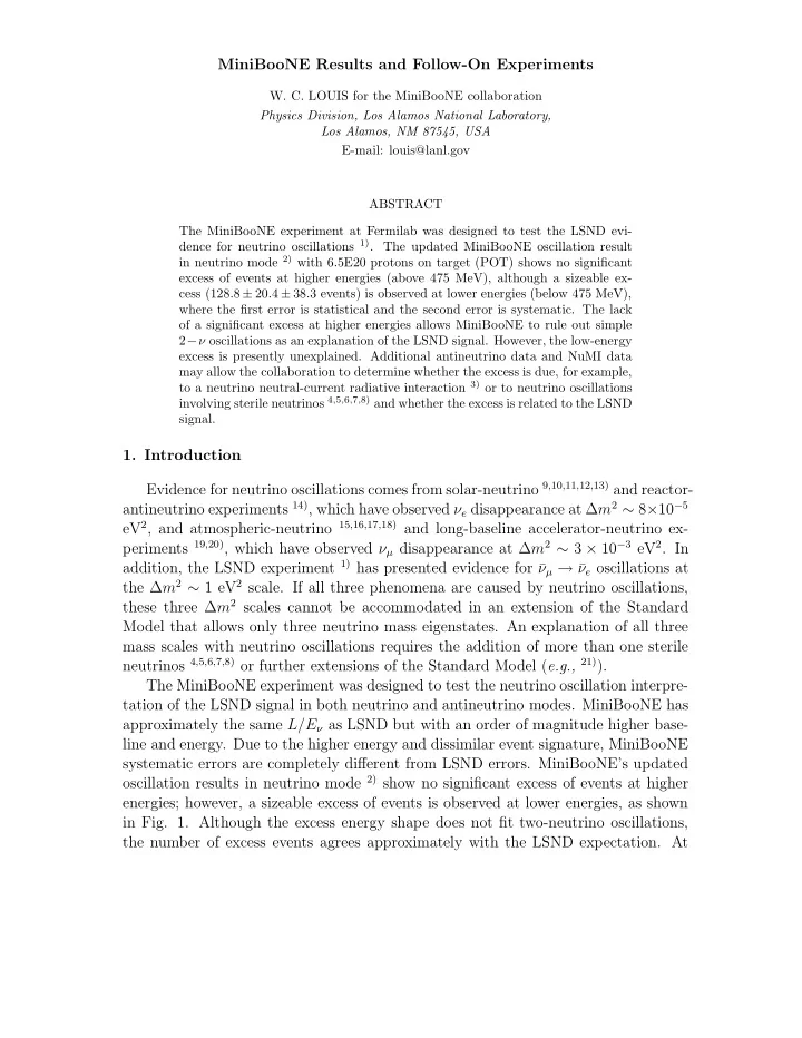
Physics Division, Los Alamos National Laboratory, Los Alamos, NM 87545, USA E-mail: louis@lanl.gov ABSTRACT The MiniBooNE experiment at Fermilab was designed to test the LSND evi- dence for neutrino oscillations 1). The updated MiniBooNE oscillation result in neutrino mode 2) with 6.5E20 protons on target (POT) shows no significant excess of events at higher energies (above 475 MeV), although a sizeable ex- cess (128.8 ± 20.4 ± 38.3 events) is observed at lower energies (below 475 MeV), where the first error is statistical and the second error is systematic. The lack
- f a significant excess at higher energies allows MiniBooNE to rule out simple
2−ν oscillations as an explanation of the LSND signal. However, the low-energy excess is presently unexplained. Additional antineutrino data and NuMI data may allow the collaboration to determine whether the excess is due, for example, to a neutrino neutral-current radiative interaction 3) or to neutrino oscillations involving sterile neutrinos 4,5,6,7,8) and whether the excess is related to the LSND signal.
Evidence for neutrino oscillations comes from solar-neutrino 9,10,11,12,13) and reactor- antineutrino experiments 14), which have observed νe disappearance at ∆m2 ∼ 8×10⁻⁵ eV2, and atmospheric-neutrino 15,16,17,18) and long-baseline accelerator-neutrino ex- periments 19,20), which have observed νµ disappearance at ∆m2 ∼ 3 × 10⁻³ eV2. In addition, the LSND experiment 1) has presented evidence for ¯ νµ → ¯ νe oscillations at the ∆m2 ∼ 1 eV2 scale. If all three phenomena are caused by neutrino oscillations, these three ∆m2 scales cannot be accommodated in an extension of the Standard Model that allows only three neutrino mass eigenstates. An explanation of all three mass scales with neutrino oscillations requires the addition of more than one sterile neutrinos 4,5,6,7,8) or further extensions of the Standard Model (e.g., 21)). The MiniBooNE experiment was designed to test the neutrino oscillation interpre- tation of the LSND signal in both neutrino and antineutrino modes. MiniBooNE has approximately the same L/Eν as LSND but with an order of magnitude higher base- line and energy. Due to the higher energy and dissimilar event signature, MiniBooNE systematic errors are completely different from LSND errors. MiniBooNE’s updated
- scillation results in neutrino mode 2) show no significant excess of events at higher
energies; however, a sizeable excess of events is observed at lower energies, as shown in Fig. 1. Although the excess energy shape does not fit two-neutrino oscillations, the number of excess events agrees approximately with the LSND expectation. At
SLIDE 2 (GeV)
QE ν
E Events / MeV
0.2 0.4 0.6 0.8 1 1.2 1.4 1.6 0.5 1 1.5 2 2.5 3
Data µ from
e
ν
+
from K
e
ν from K
e
ν misid π γ N → ∆ dirt
Total Background
1.5 3.
Figure 1: The MiniBooNE reconstructed neutrino energy distribution for candidate νe data events (points with error bars) compared to the Monte Carlo simulation (histogram).
present, with 3.4E20 POT in antineutrino mode, MiniBooNE observes no excess at lower energies.
2.1. Description of the Experiment A schematic drawing of the MiniBooNE experiment at FNAL is shown in Fig. 2. The experiment is fed by 8-GeV kinetic energy protons from the Booster that interact in a 71-cm long Be target located at the upstream end of a magnetic focusing horn. The horn pulses with a current of 174 kA and, depending on the polarity, either focuses π+ and K+ and defocuses π− and K− to form a neutrino beam or focuses π− and K− and defocuses π+ and K+ to form a less pure antineutrino beam. The produced pions and kaons then decay in a 50-m long pipe, and the resulting neutrinos and antineutrinos 22) can then interact in the MiniBooNE detector, which is located 541 m downstream of the Be target. For the MiniBooNE results presented here, a total of 6.5 × 10²⁰ POT were collected in neutrino mode and 3.4 × 10²⁰ POT were collected in antineutrino mode. The MiniBooNE detector 23) consists of a 12.2-m diameter spherical tank filled with approximately 800 tons of mineral oil (CH2). A schematic drawing of the Mini- BooNE detector is shown in Fig. 3. There are a total of 1280 8-inch detector pho- totubes (covering 10% of the surface area) and 240 veto phototubes. The fiducial
SLIDE 3 Figure 2: A schematic drawing of the MiniBooNE experiment.
MiniBooNEDetector
SignalRegion VetoRegion
Figure 3: A schematic drawing of the MiniBooNE detector.
volume has a 5-m radius and corresponds to approximately 450 tons. Only ∼ 2% of the phototube channels failed over the course of the run. 2.2. MiniBooNE Cross Section Results MiniBooNE has published two cross section results. First, MiniBooNE has made a precision measurement of νµ charged-current quasi-elastic (CCQE) scattering events
24). Fig. 4 shows the νµ CCQE Q2 distribution for data (points with error bars)
compared to a MC simulation (histograms). A strong disagreement between the data and the original simulation (dashed histogram) was first observed. However, by increasing the axial mass, MA, to 1.23±0.20 GeV and by introducing a new variable, κ = 1.019 ± 0.011, where κ is the increase in the incident proton threshold, the agreement between data and the simulation (solid histogram) is greatly improved. It
SLIDE 4 Figure 4: The νµ CCQE Q2 distribution for data (points with error bars) compared to the MC simulation (histograms).
is impressive that such good agreement is obtained by adjusting these two variables. MiniBooNE has also collected the world’s largest sample of neutral-current π0 events 25), as shown in Fig. 5. By fitting the γγ mass and Eπ(1−cos θπ) distributions, the fraction of π0 produced coherently is determined to be 19.5±1.1±2.5%. Excellent agreement is obtained between data and MC simulation. 2.3. Neutrino Oscillation Event Selection MiniBooNE searches for νµ → νe oscillations by measuring the rate of νeC → e−X CCQE events and testing whether the measured rate is consistent with the estimated background rate. To select candidate νe CCQE events, an initial selection is first applied: > 200 tank hits, < 6 veto hits, reconstructed time within the neutrino beam spill, reconstructed vertex radius < 500 cm, and visible energy Evis > 140
- MeV. It is then required that the event vertex reconstructed assuming an outgoing
electron and the track endpoint reconstructed assuming an outgoing muon occur at radii < 500 cm and < 488 cm, respectively, to ensure good event reconstruction and efficiency for possible muon decay electrons. Particle identification (PID) cuts are then applied to reject muon and π0 events. Several improvements have been made to the neutrino oscillation data analysis since the initial data was published 2), including an improved background estimate, an additional fiducial volume cut that greatly reduces the background from events produced outside the tank (dirt events),
SLIDE 5 Figure 5: The neutral-current π0 γγ mass and Eπ(1 − cos θπ) distributions for data (points with error bars) compared to the MC simulation (histograms).
and an increase in the data sample from 5.579 × 10²⁰ POT to 6.462 × 10²⁰ POT. A total of 89,200 neutrino events pass the initial selection, while 1069 events pass the complete event selection of the final analysis with EQE
ν
> 200 MeV, where EQE
ν
is the reconstructed neutrino energy. 2.4. Neutrino Oscillation Signal and Background Reactions Table 1 shows the expected number of candidate νe CCQE background events with EQE
ν
between 200−300 MeV, 300−475 MeV, and 475−1250 MeV after the complete event selection of the final analysis. The background estimate includes antineutrino events, representing < 2% of the total. The total expected backgrounds for the three energy regions are 186.8 ± 26.0 events, 228.3 ± 24.5 events, and 385.9 ± 35.7 events,
- respectively. For νµ → νe oscillations at the best-fit LSND solution of ∆m2 = 1.2
eV2 and sin2 2θ = 0.003, the expected number of νe CCQE signal events for the three energy regions are 7 events, 37 events, and 135 events, respectively. 2.5. Updated Neutrino Oscillation Results
- Fig. 1 shows the reconstructed neutrino energy distribution for candidate νe data
events (points with error bars) compared to the MC simulation (histogram) 2), while
- Fig. 6 shows the event excess as a function of reconstructed neutrino energy. Good
agreement between the data and the MC simulation is obtained for EQE
ν
> 475 MeV; however, an unexplained excess of electron-like events is observed for EQE
ν
< 475
SLIDE 6 Table 1: The expected number of events in the 200 < EQE
ν
< 300 MeV, 300 < EQE
ν
< 475 MeV, and 475 < EQE
ν
< 1250 MeV energy ranges from all of the significant backgrounds after the complete event selection of the final analysis. Also shown are the expected number of νe CCQE signal events for two-neutrino oscillations at the LSND best-fit solution.
Process 200 − 300 300 − 475 475 − 1250 νµ CCQE 9.0 17.4 11.7 νµe → νµe 6.1 4.3 6.4 NC π0 103.5 77.8 71.2 NC ∆ → Nγ 19.5 47.5 19.4 Dirt Events 11.5 12.3 11.5 Other Events 18.4 7.3 16.8 νe from µ Decay 13.6 44.5 153.5 νe from K+ Decay 3.6 13.8 81.9 νe from K0
L Decay
1.6 3.4 13.5 Total Background 186.8 ± 26.0 228.3 ± 24.5 385.9 ± 35.7 LSND Best-Fit Solution 7 ± 1 37 ± 4 135 ± 12
- MeV. As shown in Fig. 6, the magnitude of the excess is very similar to what is
expected from neutrino oscillations based on the LSND signal. Although the shape
- f the excess is not consistent with simple two-neutrino oscillations, more complicated
- scillation models 4,5,6,7,8) have shapes that may be consistent with both the LSND
and MiniBooNE signals. Table 2 shows the number of data, background, and excess events for different EQE
ν
ranges, together with the excess significance. For the final analysis, an excess
- f 128.8 ± 20.4 ± 38.3 events is observed for 200 < EQE
ν
< 475 MeV. For the entire 200 < EQE
ν
< 1250 MeV energy region, the excess is 151.0 ± 28.3 ± 50.7 events. As shown in Fig. 7, the event excess occurs for Evis < 400 MeV, where Evis is the visible energy. Figs. 8 and 9 show the event excess as functions of Q2 and cos(θ) for events in the 300 < EQE
ν
< 475 MeV range, where Q2 is determined from the energy and angle of the outgoing lepton and θ is the angle between the beam direction and the reconstructed event direction. Also shown in the figures are the expected shapes from νeC → e−X and ¯ νeC → e+X charged-current (CC) scattering and from the NC π0 and ∆ → Nγ reactions, which are representative of photon events produced by NC scattering. The NC scattering assumes the νµ energy spectrum, while the CC scattering assumes the transmutation of νµ into νe and ¯ νe, respectively. As shown in Table 3, the χ2 values from comparisons of the event excess to the expected shapes are acceptable for all of the processes. However, any of the backgrounds in Table 3 would have to be increased by > 5σ to explain the low-energy excess.
SLIDE 7 (GeV)
QE ν
E
0.2 0.4 0.6 0.8 1 1.2 1.4 1.6
Excess Events / MeV
0.2 0.4 0.6 0.8
data - expected background
e
ν →
µ
ν best-fit
2
=1.0eV
2
m ∆ =0.004, θ 2
2
sin
2
=0.1eV
2
m ∆ =0.2, θ 2
2
sin
1.5 3.
Figure 6: The event excess as a function of EQE
ν
. Also shown are the expectations from the best
- scillation fit (sin2 2θ = 0.0017, ∆m2 = 3.14 eV2) and from neutrino oscillation parameters in the
LSND allowed region. The error bars include both statistical and systematic errors.
(MeV)
vis
E
200 400 600 800 1000 1200 1400 1600 1800 2000
Excess Events / MeV
0.2 0.4 0.6 0.8 1
data - expected background
e
ν →
µ
ν best-fit
2
=1.0eV
2
m ∆ =0.004, θ 2
2
sin
2
=0.1eV
2
m ∆ =0.2, θ 2
2
sin
Figure 7: The event neutrino excess as a function of Evis for EQE
ν
> 200 MeV. Also shown are the expectations from the best oscillation fit (sin2 2θ = 0.0017, ∆m2 = 3.14 eV2) and from neutrino
- scillation parameters in the LSND allowed region.
The error bars include both statistical and systematic errors.
SLIDE 8 Table 2: The number of data, background, and excess events for different EQE
ν
ranges, together with the significance of the excesses in neutrino mode.
Event Sample Final Analysis 200 − 300 MeV Data 232 Background 186.8 ± 13.7 ± 22.1 Excess 45.2 ± 13.7 ± 22.1 Significance 1.7σ 300 − 475 MeV Data 312 Background 228.3 ± 15.1 ± 19.3 Excess 83.7 ± 15.1 ± 19.3 Significance 3.4σ 200 − 475 MeV Data 544 Background 415.2 ± 20.4 ± 38.3 Excess 128.8 ± 20.4 ± 38.3 Significance 3.0σ 475 − 1250 MeV Data 408 Background 385.9 ± 19.6 ± 29.8 Excess 22.1 ± 19.6 ± 29.8 Significance 0.6σ
)
2
(GeV
2
Q
0.05 0.1 0.15 0.2 0.25 0.3 0.35 0.4 0.45 0.5
/1000 )
2
Excess Events / ( GeV
0.2 0.4 0.6 0.8 1
data - expected background background shape π background shape ∆ signal shape
e
ν signal shape
e
ν Figure 8: The neutrino event excess as a function of Q2 for 300 < EQE
ν
< 475 MeV.
SLIDE 9 ) θ cos(
0.2 0.4 0.6 0.8 1
Excess Events
10 20 30 40 50
data - expected background background shape π background shape ∆ signal shape
e
ν signal shape
e
ν
Figure 9: The neutrino event excess as a function of cos(θ) for 300 < EQE
ν
< 475 MeV. Table 3: The χ2 values from comparisons of the neutrino event excess Q2 and cos(θ) distributions for 300 < EQE
ν
< 475 MeV to the expected shapes from various NC and CC reactions. Also shown is the factor increase necessary for the estimated background for each process to explain the low-energy excess.
Process χ2(cosθ)/9 DF χ2(Q2)/6 DF Factor Increase NC π0 13.46 2.18 2.0 ∆ → Nγ 16.85 4.46 2.7 νeC → e−X 14.58 8.72 2.4 ¯ νeC → e+X 10.11 2.44 65.4
SLIDE 10 Figure 10: The estimated neutrino fluxes for neutrino mode (top plot) and antineutrino mode (bottom plot).
2.6. Initial Antineutrino Oscillation Results The same analysis that was used for the neutrino oscillation results is employed for the initial antineutrino oscillation results 26). Fig. 10 shows the estimated neutrino fluxes for neutrino mode and antineutrino mode, respectively. The fluxes are fairly similar (the intrinsic electron-neutrino background is approximately 0.5% for both modes of running), although the wrong-sign contribution to the flux in antineutrino mode (∼ 18%) is much larger than in neutrino mode (∼ 6%). The average νe plus ¯ νe energies are 0.96 GeV in neutrino mode and 0.77 GeV in antineutrino mode, while the average νµ plus ¯ νµ energies are 0.79 GeV in neutrino mode and 0.66 GeV in antineu- trino mode. Also, as shown in Fig. 11, the estimated backgrounds in the two modes are very similar, especially at low energy. Fig. 12 shows the expected antineutrino
- scillation sensitivity for the present data sample corresponding to 3.4E20 POT. The
two sensitivity curves correspond to threshold neutrino energies of 200 MeV and 475 MeV. The initial oscillation results for antineutrino mode are shown in Table 4 and
- Figs. 13 through 15. It is quite surprising that no excess (−0.5 ± 7.8 ± 8.7 events)
SLIDE 11
Figure 11: The estimated backgrounds for the neutrino oscillation search in neutrino mode (top plot) and antineutrino mode (bottom plot). The π0, ∆ → Nγ, intrinsic νe/¯ νe, external event, and other backgrounds correspond to the green, pink, light blue, blue, and yellow colors, respectively. Figure 12: The expected antineutrino oscillation sensitivity at 90% CL for the present data sample corresponding to 3.4E20 POT. The two sensitivity curves correspond to threshold energies of 200 MeV (red curve) and 475 MeV (black curve).
SLIDE 12 is observed in the low-energy range 200 < EQE
ν
< 475 MeV. In order to understand the implications that the antineutrino data have on the neutrino low-energy excess, Table 5 shows the expected excess of low-energy events in antineutrino mode under various hypotheses. These hypotheses include the following:
- Same σ: Same cross section for neutrinos and antineutrinos.
- π0 Scaled: Scaled to number of neutral-current π0 events.
- POT Scaled: Scaled to number of POT.
- BKGD Scaled: Scaled to total background events.
- CC Scaled: Scaled to number of charged-current events.
- Kaon Scaled: Scaled to number of low-energy kaon events.
- Neutrino Scaled: Scaled to number of neutrino events.
Also shown in the Table is the probability (from a two-parameter fit to the data) that each hypothesis explains the observed number of low-energy neutrino and an- tineutrino events, assuming only statistical errors, correlated systematic errors, and uncorrelated systematic errors. A proper treatment of the systematic errors is in progress; however, it is clear from the Table that the “Neutrino Scaled” hypothe- sis fits best and that the “Same σ”, “POT Scaled”, and “Kaon Scaled” hypotheses are strongly disfavored. It will be very important to understand this unexpected difference between neutrino and antineutrino properties. The antineutrino data were also fit for oscillations in the energy range 475 < EQE
¯ ν
< 3000 MeV, assuming antineutrino oscillations but no neutrino oscillations. The antineutrino oscillation allowed region is shown in Fig. 16. At present, the
- scillation limit is worse than the sensitivity. The best oscillation fit corresponds to
∆m2 = 4.4 eV2, sin2 2θ = 0.0047, and a fitted excess of 18.6 ± 13.2 events, which is consistent with the LSND best fit point of ∆m2 = 1.2 eV2, sin2 2θ = 0.003, and an expected excess of 14.7 events. With the present antineutrino statistics, the data are consistent with both the LSND best-fit point and the null point, although the LSND best-fit point has a better χ2 (χ2 = 17.63/15 DF, probability = 30%) than the null point (χ2 = 22.19/15 DF, probability = 10%). 2.7. MiniBooNE NuMI Results Neutrino events are also observed in MiniBooNE from the NuMI beam 27). The NuMI beam, as shown in Fig. 17, differs from the Booster neutrino beam (BNB) in several respects. First, the NuMI beam is off axis by 110 mrad, whereas the BNB is on axis. Second, neutrinos from NuMI travel ∼ 700 m, compared to ∼ 500 m for
SLIDE 13 Table 4: The number of antineutrino data, background, and excess events for different EQE
¯ ν
ranges, together with the significance of the excesses in antineutrino mode.
Event Sample Final Analysis 200 − 475 MeV Data 61 Background 61.5 ± 7.8 ± 8.7 Excess −0.5 ± 7.8 ± 8.7 Significance −0.04σ 475 − 1250 MeV Data 61 Background 57.8 ± 7.6 ± 6.5 Excess 3.2 ± 7.6 ± 6.5 Significance 0.3σ 475 − 3000 MeV Data 83 Background 77.4 ± 8.8 ± 9.6 Excess 5.6 ± 8.8 ± 9.6 Significance 0.4σ
Figure 13: The comparison between data and Monte Carlo expectation as a function of reconstructed neutrino energy for the present antineutrino data sample corresponding to 3.4E20 POT.
SLIDE 14 Figure 14: The comparison between data and Monte Carlo expectation (top) and the excess number
- f events (bottom) as a function of reconstructed neutrino energy for the present antineutrino data
sample corresponding to 3.4E20 POT. Also shown are the expectations from the best oscillation fit and from oscillation parameters in the LSND allowed region.
SLIDE 15 (MeV)
vis
E
200 400 600 800 1000 1200 1400 1600 1800 2000
Excess Events / MeV
0.05 0.1 0.15 0.2 0.25
data - expected background
e
ν →
µ
ν best-fit
2
=1.0eV
2
m ∆ =0.004, θ 2
2
sin
2
=0.1eV
2
m ∆ =0.2, θ 2
2
sin
Figure 15: The excess number of events (data minus Monte Carlo expectation) as a function of visible energy for the present antineutrino data sample corresponding to 3.4E20 POT. Also shown are the expectations from the best oscillation fit and from oscillation parameters in the LSND allowed region. Table 5: The expected excess of low-energy events in antineutrino mode under various hypotheses for 3.4E20 POT. Also shown in the Table is the probability (from a two-parameter fit to the data) that each hypothesis explains the observed number of low-energy neutrino and antineutrino events, assuming only statistical errors, correlated systematic errors, and uncorrelated systematic errors.
Hypothesis # of ¯ ν Events
- Stat. Err.
- Cor. Syst. Err.
- Uncor. Syst. Err.
Same σ 37.2 0.1% 0.1% 6.7% π0 Scaled 19.4 3.6% 6.4% 21.5% POT Scaled 67.5 0.0% 0.0% 1.8% BKGD Scaled 20.9 2.7% 4.7% 19.2% CC Scaled 20.4 2.9% 5.2% 19.9% Kaon Scaled 39.7 0.1% 0.1% 5.9% Neutrino Scaled 6.7 38.4% 51.4% 58.0%
SLIDE 16 Figure 16: The antineutrino oscillation allowed region in the energy range 475 < EQE
¯ ν
< 3000 MeV for the present antineutrino data sample corresponding to 3.4E20 POT. Also shown are the best
- scillation fit (∆m2 = 4.4 eV2, sin2 2θ = 0.0047, corresponding to an excess of 18.6 ± 13.2 events)
and the LSND best fit point (∆m2 = 1.2 eV2, sin2 2θ = 0.003, corresponding to an excess of 14.7 events).
SLIDE 17
Figure 17: The NuMI beam.
neutrinos from the BNB. Also, the NuMI beam has a 6% contribution from electron- neutrinos and a 14% contribution from antineutrinos, while the BNB percentages are 0.5% and 2%, respectively. Fig. 18 shows the estimated neutrino flux at the MiniBooNE detector from the NuMI beam, while Fig. 19 compares the neutrino fluxes from the BNB and NuMI beams. Figs. 20 and 21 show the comparison between data events (points with error bars) and the MC simulation (histogram) for νµ CCQE candidate events and νe CCQE candidate events, respectively. Although the systematic errors are presently large, the data are observed to be systematically low for νµ CCQE candidate events and systematically high for νe CCQE candidate events. Updated results should be available soon with three times the data sample and with reduced systematic errors by constraining the normalization to the νµ sample. The NuMI data analysis is currently directed toward examining the low-energy region and searching for neutrino oscillations. This will complement the analysis done with MiniBooNE using neutrino and anti-neutrino BNB data, but with different systematic errors. It is worth noting that the NuMI νe CCQE sample has a very different composition when compared to the BNB neutrino νe CCQE sample. The BNB νe CCQE sample originates mostly from decays of pions and muons and contains a large fraction of νµ-induced mis-identified events. On other hand, the NuMI νe
SLIDE 18 [GeV]
ν
E
0.5 1 1.5 2 2.5 3 3.5 4
]
2
/POT/GeV/cm ν ) [
ν
(E Φ
10
10
10 1
µ
ν
µ
ν
e
ν
e
ν
Figure 18: The estimated neutrino flux at the MiniBooNE detector from the NuMI beam.
[GeV]
ν
E 0.5 1 1.5 2 2.5 3 3.5 4 4.5 5 /50MeV]
2
POT)/m
6
/(10 ν [
ν
Φ
10
10 1 π K
L
K NuMI On-axis Flux (at MINOS) NuMI Off-axis Flux (at MinibooNE) BNB On-axis Flux (at MinibooNE)
Figure 19: A comparison between the BNB and NuMI neutrino fluxes.
SLIDE 19
[GeV]
ν
Reconstructed E
0.2 0.7 1.2 1.7 2.2
Events/(100 MeV)
1000 2000 3000 Data Spectrum
µ
ν Predicted Uncertainty in Prediction Neutrinos from K’s ’s π Neutrinos from
Figure 20: The comparison between data events (points with error bars) and the MC simulation (histogram) for NuMI-induced νµ CCQE candidate events.
[GeV]
ν
Reconstructed E
0.2 0.6 1 1.4 1.8 2.2 2.6 3
Events/(100 MeV)
20 40 60 80 Data Spectrum
e
ν Predicted Uncertainty in Prediction ’s
±
Neutrinos from K ’s
L
Neutrinos from K ’s µ Neutrinos from ’s π Neutrinos from
Figure 21: The comparison between data events (points with error bars) and the MC simulation (histogram) for NuMI-induced νe CCQE candidate events.
SLIDE 20 CCQE sample is produced mostly from the decay of kaons and contains a dominant fraction of intrinsic νe events. The analysis will be done by forming a correlation between the νµ CCQE and νe CCQE samples and by tuning the prediction to the data simultaneously. The result is that common systematics cancel, and this might reveal something important about the nature of the νe sample.
- 3. Physics Goals with 1E21 POT in Antineutrino Mode
MiniBooNE, so far, has collected ∼ 6.5 × 10²⁰ POT in neutrino mode and ∼ 3.4 × 10²⁰ POT in antineutrino mode. For the future, it is imperative to understand the MiniBooNE low-energy excess and to determine whether there is an unexpected difference between neutrino and antineutrino properties. The event excess in neutrino mode (and the apparent lack of an excess in antineutrino mode) is very interesting in its own right and important for future long-baseline experiments such as T2K, NOνA, and LBNE. T2K will have a very similar neutrino energy distribution to MiniBooNE and will, therefore, be affected by the same low-energy excess. In addition, it is very important to test directly the LSND signal with a higher statistics antineutrino data sample. 3.1. Testing the Low-Energy Excess with Antineutrinos With 1E21 POT in antineutrino mode, MiniBooNE will be able to determine con- clusively whether there is an anomalous difference between neutrino and antineutrino
- properties. Table 6 shows the expected excess of low-energy events in antineutrino
mode under various hypotheses for 1E21. Also shown in the Table is the probability (from a two-parameter fit to the data and assuming no excess in antineutrino mode) that each hypothesis explains the observed number of low-energy neutrino and an- tineutrino events, assuming only statistical errors, correlated systematic errors, and uncorrelated systematic errors. As can be seen in Table 6, the Neutrino Scaled hy- pothesis can be verified (and the other hypotheses rejected) with 1E21 POT if no excess is observed in antineutrino mode. 3.2. A Direct Test of the LSND signal with Antineutrinos With 1E21 POT in antineutrino mode, MiniBooNE will be able to make a direct and fairly sensitive test of the LSND signal. For the best-fit LSND point of ∆m2 = 1.2 eV2 and sin2 2θ = 0.003 1), MiniBooNE should observe in the 475 < EQE
ν
< 3000 MeV energy range an excess of ∼ 40.0±15.2±20.9 events, corresponding to a ∼ 1.5σ
- signal. The significance of such a signal may be improved by further reductions in the
systematic uncertainties (e.g. by comparing antineutrino data to neutrino data). Fig. 22 shows the expected antineutrino oscillation sensitivity for a threshold energy of
SLIDE 21 Table 6: The expected excess of low-energy events in antineutrino mode under various hypotheses for 1E21 POT. Also shown in the Table is the probability (from a two-parameter fit to the data and assuming no excess in antineutrino mode) that each hypothesis explains the observed number of low-energy neutrino and antineutrino events, assuming only statistical errors, correlated systematic errors, and uncorrelated systematic errors.
Hypothesis # of ¯ ν Events
- Stat. Err.
- Cor. Syst. Err.
- Uncor. Syst. Err.
Same σ 111.6 0.0% 0.0% 4.7% π0 Scaled 58.2 0.1% 1.4% 17.1% POT Scaled 202.5 0.0% 0.0% 1.3% BKGD Scaled 62.7 0.1% 0.8% 15.0% CC Scaled 61.2 0.1% 1.0% 15.6% Kaon Scaled 119.1 0.0% 0.0% 4.0% Neutrino Scaled 20.1 17.2% 44.1% 54.5% 475 MeV. The curves correspond to 3.4E20 POT, 5E20 POT, and 1E21 POT. With 1E21 POT, most of the LSND region is covered at 90% CL. 3.3. MiniBooNE Follow-On For the future, it will be imperative to understand the MiniBooNE low-energy
- excess. This excess is very interesting in its own right and important for future long-
baseline experiments such as T2K, NOνA, and LBNE. T2K will have a very similar neutrino energy distribution to MiniBooNE and will, therefore, be affected by the same low-energy excess. By analyzing the MiniBooNE antineutrino data, NuMI data, and SciBooNE data, it may be possible to reduce systematic errors and determine whether any of the published models 3,4,5,6,7,8) can provide an explanation for the
- excess. A full error matrix with correlated and uncorrelated systematic errors is used
to estimate the systematic error at low energies and includes errors from neutrino flux, neutrino cross sections, and detector response. By comparing data sets, some of these systematic errors will cancel. If the low-energy excess continues to be consistent with a signal, then new experiments at FNAL (MicroBooNE and BooNE) or ORNL (OscSNS) should be built to explore physics beyond the Standard Model.
The MicroBooNE experiment 28), which was recently approved at Fermilab, ex- ploits the precise differentiation of photons versus electrons in a detector, as is uniquely available from a Liquid Argon Time Projection Chamber (LArTPC). The detector consists of a ∼ 70 ton fiducial volume LArTPC. It will run near the Mini- BooNE enclosure on the BNB with an expected exposure of 6×10²⁰ protons on target. Approximately 105 events will be collected with the BNB and about 6 × 10⁴ events
SLIDE 22 ) θ (2
2
sin
10
10
10 1
2
m ∆
10
10 1 10
2
10
3.386E20 POT 5.0E20 POT 10.0E20 POT
Figure 22: The expected antineutrino oscillation sensitivity for a threshold energy of 475 MeV. The curves correspond to 3.4E20 POT, 5E20 POT, and 1E21 POT.
with the off-axis NuMI beam. The high spatial resolution and energy measurement down to the MeV scale will substantially improve on information available from the MiniBooNE detector. The experiment will run in 2011. The MicroBooNE detector, as shown in Fig. 23, can separate electron showers from photon showers using the energy deposited in the first 2.4 cm of the track. For an electron efficiency of 80%, γ contamination is expected to be < 5%, based on MC
- studies. The electron and γ energy resolution is < 10% for energies above 15 MeV.
Given the excellent e/γ separation, MicroBooNE can identify the source of the low energy events observed in MiniBooNE. MicroBooNE’s sensitivity to the low energy excess is ∼ 5σ if the signal is electron-like and ∼ 3σ if the signal is photon-like, in a strictly counting-based experiment. Fits to shape-signatures may increase the significance.
The BooNE experiment would involve building a second detector at a cost of ∼ $8M along the BNB at FNAL at a different distance. With two detectors, many
- f the systematic errors would cancel, as the neutrino flux varies as 1/r2 to good
approximation, so that a simple ratio of events in the two detectors would provide a sensitive search for νe appearance and νµ disappearance. Furthermore, by comparing the rates for a NC reaction, such as NC π0 scattering or NC elastic scattering, a
SLIDE 23 Figure 23: A schematic drawing of the MicroBooNE detector.
sensitive search for sterile neutrinos can be made. An even cheaper option would be to move the MiniBooNE detector to a different location at a cost of only ∼ $3M. For example, if the MiniBooNE detector were moved to a distance of 200 m from the neutrino source, then the event rate would increase by a factor of ∼ 6 due to the 1/r2 dependence of the neutrino flux. After a year
- f running, the comparison of the event rates at the two locations could determine
whether the low-energy excess observed by MiniBooNE was due to neutrino oscilla-
- tions. In addition, νµ and ¯
νµ disappearance could be searched for with high precision in the ∆m2 > 0.1 eV2 mass region.
The OscSNS experiment 29) would involve building a MiniBooNE-like detector at a distance of ∼ 60 m from the SNS beam dump at ORNL. The detector would be the same as MiniBooNE except with a higher phototube coverage of 25% and the addition
- f ∼ 0.031 g/l of butyl-PBD scintillator. Due to the higher phototube coverage, the
estimated cost is ∼ $12M. Fig. 24 shows the layout of the SNS, which is running with a proton energy of 1 GeV with a goal of eventually reaching a beam power of ∼ 1.4
- MW. The great advantage of the SNS is that the neutrino flux is extremely intense
and known almost perfectly, and the neutrino cross sections are known well. Fig. 25 shows the neutrino flux energy distribution, which includes a monoenergetic 30 MeV
SLIDE 24 Figure 24: The layout of the SNS.
νµ from π+ DAR and νe and ¯ νµ from µ+ DAR. Furthermore, as shown in the left plot
- f Fig. 25, the monoenergetic νµ can be identified by timing, as was performed by
the KARMEN experiment at the ISIS proton accelerator. With the SNS neutrino flux, OscSNS would be capable of making precision mea- surements of νe and ¯ νe appearance and νµ disappearance and proving the existence
- f sterile neutrinos via the NC reaction νµC → νµC∗(15.11). Any observed reduction
- f this cross section would be evidence for active-sterile neutrino oscillations. Fig.
26 shows the expected active-sterile neutrino oscillation sensitivity as a function of ∆m2 and sin2 2θ 29). Fig. 27 shows the expected ¯ νe appearance sensitivity. Other physics goals include precision measurements of νe → νe elastic scattering (and the world’s best sensitivity for the νµ magnetic moment) and νeC → e−N charged-current scattering.
The MiniBooNE experiment observes an unexplained excess of electron-like events at low energies in neutrino mode, which may be due, for example, to either a neutral current radiative interaction 3) or to neutrino oscillations involving sterile neutrinos
4,5,6,7,8) and which may be related to the LSND signal. No excess of electron-like
events, however, is observed so far at low energies in antineutrino mode. MiniBooNE, therefore, has requested additional running in antineutrino mode for a total of 1E21
SLIDE 25 Figure 25: The right plot shows the neutrino flux energy distribution, which includes a monoenergetic 30 MeV νµ from π+ DAR and νe and ¯ νµ from µ+ DAR. The left plot shows the neutrino time
- distribution. The monoenergetic νµ can be identified by timing.
Figure 26: The expected OscSNS active-sterile neutrino oscillation sensitivity as a function of ∆m2 and sin2 2θ after three years of data taking.
SLIDE 26 Figure 27: The expected OscSNS ¯ νµ → ¯ νe oscillation sensitivity as a function of ∆m2 and sin2 2θ after three years of data taking.
- POT. With this additional data taking, which should be completed by the end of
2011, the MiniBooNE collaboration will be able to determine conclusively whether there is an anomalous difference between neutrino and antineutrino properties. In addition, the high energy antineutrino data will provide a direct test of the LSND signal and will increase the statistics of the NuMI data sample. With the present 3.4E20 POT in antineutrino mode, almost all of the LSND region is still allowed, as the current limit is worse than the sensitivity. However, with 1E21 POT in the case of no neutrino oscillations, most of the LSND allowed region should be ruled out. In the case of neutrino oscillations at the LSND best-fit point, a ∼ 1.5σ event excess would be expected. If the low-energy excess continues to be consistent with a signal, then new exper- iments at FNAL (MicroBooNE and BooNE) or ORNL (OscSNS) should be built to explore physics beyond the Standard Model.
We thank Milla Baldo Ceolin for the invitation to make a presentation at this stimulating conference and for her superb organization of the conference.
SLIDE 27 1) C. Athanassopoulos et al., Phys. Rev. Lett. 75, 2650 (1995); 77, 3082 (1996); 81, 1774 (1998); A. Aguilar et al., Phys. Rev. D 64, 112007 (2001). 2) A. Aguilar-Arevalo et al., Phys. Rev. Lett. 98, 231801 (2007); A. Aguilar- Arevalo et al., Phys. Rev. Lett. 102, 101802 (2009). 3) Jeffrey A. Harvey, Christopher T. Hill, Richard J. Hill, [arXiv:0708.1281]; [arXiv:0712.1230]. 4) Michel Sorel, Janet Conrad, and Michael Shaevitz, Phys. Rev. D 70, 073004 (2004); C. Karagiorgi et al., Phys. Rev. D 75, 013011 (2007); Alessandro Melchiorri et al., [arXiv:0810.5133]. 5) Heinrich Paes, Sandip Pakvasa, Thomas J. Weiler, Phys. Rev. D 72, 095017 (2005); [arXiv:hep-ph/0504096]. 6) T. Goldman, G. J. Stephenson Jr., and B. H. J. McKellar, Phys. Rev. D 75, 091301 (2007). 7) Michele Maltoni and Thomas Schwetz, Phys. Rev. D 76, 093005 (2007); [arXiv:0705.0197]. 8) Ann E. Nelson and Jonathan Walsh, [arXiv:0711.1363]. 9) B. T. Cleveland et al., Astrophys. J. 496, 505 (1998). 10) J. N. Abdurashitov et al., Phys. Rev. C 60, 055801 (1999). 11) W. Hampel et al., Phys. Lett. B 447, 127 (1999). 12) S. Fukuda et al., Phys. Lett. B 539, 179 (2002). 13) Q. R. Ahmad et al., Phys. Rev. Lett. 87, 071301 (2001); Q. R. Ahmad et al.,
- Phys. Rev. Lett. 89, 011301 (2002); S. N. Ahmed et al., Phys. Rev. Lett. 92,
181301 (2004). 14) K. Eguchi et al., Phys. Rev. Lett. 90, 021802 (2003); T. Araki et al., Phys.
- Rev. Lett. 94, 081801 (2005).
15) K. S. Hirata et al., Phys. Lett. B 280, 146 (1992); Y. Fukuda et al., Phys.
16) Y. Fukuda et al., Phys. Rev. Lett. 81, 1562 (1998). 17) W. W. M. Allison et al., Phys. Lett. B 449, 137 (1999). 18) M. Ambrosio et al., Phys. Lett. B 517, 59 (2001). 19) M. H. Ahn et al., Phys. Rev. Lett. 90, 041801 (2003). 20) D. G. Michael et al., Phys. Rev. Lett. 97, 191801 (2006); P. Adamson et al.,
- Phys. Rev. Lett. 101, 131802 (2008).
21) T. Katori, A. Kostelecky and R. Tayloe, Phys. Rev. D 74, 105009 (2006). 22) A. Aguilar-Arevalo et al., [arXiv:0806.1449]. 23) A. Aguilar-Arevalo et al., Nucl. Instr. Meth. A559, 28 (2009). 24) A. Aguilar-Arevalo et al., Phys. Rev. Lett. 100, 032301 (2008). 25) A. Aguilar-Arevalo et al., Phys. Lett. 664B, 41 (2008). 26) A. Aguilar-Arevalo et al., [arXiv:0904.1958]. 27) P. Adamson et al., [arXiv:0809.2447]. 28) H. Chen et al., A Proposal for a New Experiment Using the Booster and NuMI Neutrino Beamlines: MicroBooNE (2007). 29) G. T. Garvey et al., Phys. Rev. D 72, 092001 (2005).