Michelson-Morley, Fisher, and Occam: The Radical Implications of - PowerPoint PPT Presentation
Michelson-Morley, Fisher, and Occam: The Radical Implications of Stable Inflation at the Zero bound Also Stepping on a Rake: the Fiscal Theory of Monetary Policy John H. Cochrane Hoover Institution, Stanford University October 2017
Michelson-Morley, Fisher, and Occam: The Radical Implications of Stable Inflation at the Zero bound – Also – Stepping on a Rake: the Fiscal Theory of Monetary Policy John H. Cochrane Hoover Institution, Stanford University October 2017 1 / 34
Michelson-Morley; The long quiet ZLB 6 5 10Y Govt 4 Core CPI 3 2 1 Fed Funds Reserves 0 1996 1998 2000 2002 2004 2006 2008 2010 2012 2014 2016 ◮ What happens at the ZLB? Nothing . 2 / 34
Michelson-Morley; The long quiet ZLB 6 5 10Y Govt 4 3 Core CPI 2 1 Fed Funds Reserves 0 1996 1998 2000 2002 2004 2006 2008 2010 2012 2014 2016 ◮ Quiet, stable π at long period of i ≈ 0, φ << 1, huge M . ◮ No deflation spiral. No M/QE inflation. No sunspot volatility. No change in π dynamics. σ ( π ) lower? 3 / 34
US unemployment and GDP 10 Unemployment 8 6 4 Fed Funds 2 0 GDP Growth -2 1994 1996 1998 2000 2002 2004 2006 2008 2010 2012 2014 2016 ◮ Larger shock but same dynamics. Faster decline in u, lower σ (∆ Y )? E (∆ Y ) is too low, but is that monetary policy? 4 / 34
Japan 6 5 4 3 Percent 10Y Govt 2 1 Int rate 0 -1 Core CPI -2 1992 1994 1996 1998 2000 2002 2004 2006 2008 2010 2012 2014 2016 ◮ 20+ years at i ≈ 0 with no spiral, sunspot σ ( π ). ◮ Spiral fear understandable in 2001. 5 / 34
Europe 5 1 mo Euro Libor 4 3 Percent 2 Euro Core CPI 1 0 -1 2000 2002 2004 2006 2008 2010 2012 2014 2016 ◮ Lower rates ↔ lower inflation. 6 / 34
Core Monetary Doctrines / ZLB predictions ◮ Old K/Adaptive E: ZLB → Deflation spiral. ◮ (Friedman 68) ZLB, i peg, or passive φ is unstable . π t +1 = ( λ > 1) π t + shocks. ◮ Taylor φ > 1 stabilizes. ZLB → φ < 1. ◮ NK/Rational E: ZLB → π is stable but volatile ; ◮ “Self-confirming fluctuations,” “sunspots.” E t π t +1 = ( λ ≤ 1) π t ; π t +1 = E t π t +1 + δ t +1 . ◮ Taylor φ > 1 makes unstable, hence determinate. ◮ φ < 1 volatility a core prediction. 70/80; Japan ZLB. ◮ MV=PY: ZLB, i ≈ 0 is irrelevant. M $50b → $3,000b means hyperinflation . Velocity is “stable.” QE “injects liquidity.” 7 / 34
Simple models x t = E t x t +1 − σ ( r t − v r t ) IS i t = r t + π e Fisher t π t = π e t + κ x t Phillips i t = φπ t + v i Slides t r ∗ + π ∗ + φ ( π t − π ∗ ) + v i � � i t = max t , 0 Taylor Eliminate i t , r t , x t , (1 + φσκ ) π t = (1 + σκ ) π e t + σκ ( v r t − v i t ) Old Keynesian, π e t = π t − 1 ; φ < 1 unstable: π t = 1 + σκ σκ 1 + φσκ ( v r t − v i 1 + φσκπ t − 1 + t ) New Keynesian π e t = E t π t +1 , ; φ < 1 stable, indeterminate: E t π t +1 = 1 + φσκ σκ 1 + σκ ( v i t − v r 1 + σκ π t + t ) . 8 / 34
Adaptive/Old-Keynesian Spiral 4 i 2 π 0 Percent -2 v r -4 -6 -8 -10 -12 -2 0 2 4 6 8 10 Time t ); π t = π t − 1 + κ x t ; i t = max[ i ∗ + φ ( π t − π ∗ ) , 0] x t = − σ ( i t − π t − 1 − v r 9 / 34
Rational E / New-Keynesian stable but indeterminate 3 2 1 E t π t+1 0 -1 -2 -3 -3 -2 -1 0 1 2 3 π t E t ( π t +1 − π ∗ ) = 1 + φσκ 1 σκ 1 + σκ ( π t − π ∗ ) / E t π t +1 = 1 + σκπ t − 1 + σκ r 10 / 34
Michelson-Morley Michelson-Morley. Experiment: ◮ Inflation can be stable, quiet, at ZLB, φ < 1. Even a peg. ◮ Huge excess reserves paying market interest are not inflationary. ◮ φ > 1 vs. φ < 1, ZLB, is not a key state variable for σ ( π ), dynamics. Implications ◮ Old-Keynesian. No spiral. ◮ New-Keynesian. No sunspots. ◮ MV=PY. No hyperinflation. Next theory? New Keynesian + Fiscal Theory. ◮ Inflation can be stable and determinate , (quiet) at ZLB, φ < 1, and even a peg. 11 / 34
NK + FTPL ∞ B t − 1 � β j s t + j = E t P t j =0 � P t ∞ � B t � β j s t +1+ j . ( E t +1 − E t ) = ( E t +1 − E t ) (1) P t P t +1 j =0 ◮ Unexpected deflation ↔ debt worth more ↔ raise tax/cut spending. ◮ (1) solves spiral, indeterminacy/sunspots. δ t +1 = π t +1 − E t π t +1 ↔ fiscal policy. ◮ i peg or φ < 1 can be stable (NK) and (now) determinate and quiet . ◮ NK + FTPL is the only existing, simple, economic, theory left. ◮ Fiscal theory lite. 12 / 34
Occam: The (Long) Paper What about... ◮ Variations to rescue instability, indeterminacy, M? (A: epicycles.) ◮ Really unstable but QE offset deflation spiral? ◮ NK Equilibrium selection from post-bound actions, not current φπ t ? ◮ Really active NK, not expected to last? (A: 7 Tails? Japan?) ◮ Really unstable but slow to emerge (sticky wages, velocity)? ◮ Reserves didn’t leak to M1, M2. My point exactly. ◮ More general models? (A: don’t change stability, determinacy.) ◮ Fiscal theory objections? ◮ Large deficits, debt, Japan? (A: Low r . Not deficits, debt ↔ π .) ◮ Previous pegs, 1970/1980, other episodes? (A: Fiscal problems. “A peg can be stable.”) ◮ Why is σ ( π ) = σ (E fiscal policy) low? (“A peg can be quiet”) ◮ “Budget constraint,” debt repayment means passive fiscal? (A: No; off equilibrium modeling just like NK.) ◮ “Exogenous” surpluses? s = τ y ? s ( P )? (A: No. Like dividends.) ◮ Test FTPL? (A: Test MV=PY? P = EPV(D)?) ◮ A: Today: I only claim FTPL is possible , survives quiet ZLB test. I do not claim it proved , explains all history. 13 / 34
Selection by future active policy Interest rate Inflation 10 10 v r = -2 v r = 0 9 8 v r = -2 v r = 0 8 6 7 4 6 2 5 percent percent 0 4 -2 3 -4 2 -6 1 -8 0 -10 -1 0 5 10 15 0 5 10 15 time time ◮ φ = 0 now, but expected φ in the far future can select equilibria. ◮ People expect the Fed to destabilize? ◮ Back to trap equilibria are still there. ◮ Puzzles. Jump at t = 0. Backward stable paradoxes. ◮ Small ∆ E t π T have big effects, volatility? ◮ Is all monetary policy just talk about future threats? Why not 70s? ◮ FTPL stops jump at 0, selects benign equilibrium, solves paradoxes. 14 / 34
Fisher ◮ If π is stable at zero bound, hence peg, then if the Fed raises i , permanently, then π should eventually rise . ◮ Unavoidable consequence of stability. ◮ Vs. Friedman 1968 spiral. ◮ π could still decline in the short run . Does it? 15 / 34
Frictionless model 1.5 1.5 interest rate i interest rate i Standard NK → 1 1 0.5 0.5 Percent response Percent response inflation π inflation π 0 0 -0.5 -0.5 π with fiscal shocks π , with fiscal shocks -1 -1 also π with long term debt also π with long term debt -1.5 -1.5 -3 -2 -1 0 1 2 3 -5 -4 -3 -2 -1 0 1 2 3 Time Time ◮ Model i t = r + E t π t +1 , � β j s t + j / ( B / P ) π t +1 − E t π t +1 = ( E t +1 − E t ) ◮ “Monetary policy” changes i with no change in fiscal { s } . ◮ Higher i raises π , immediately. Pricing frictions give a temporary negative π ? ... 16 / 34
Effects of rate rise – Standard NK model with φ = 0 interest rate i 1 0.8 inflation π 0.6 0.4 Percent response 0.2 0 -0.2 output gap x -0.4 -0.6 -0.8 -1 -4 -2 0 2 4 6 Time ◮ x t = E t x t +1 − σ ( i t − E t π t +1 ); π t = β E t π t +1 + κ x t . ◮ Pricing frictions do not produce π decline. 17 / 34
Standard NK model with φ > 1 (Woodford) ρ = 1 ρ = 0.9 i π 2 1.5 π i 1.5 Percent (%) Percent (%) 1 1 0.5 0.5 0 0 -0.5 -0.5 v i v i -1 -1 0 2 4 6 8 10 0 2 4 6 8 10 Time Time ρ = 1/ λ 1 : 0.51 ρ = 0.3 0.5 0.5 π Percent (%) Percent (%) π 0 i 0 i -0.5 -0.5 v i v i -1 -1 0 2 4 6 8 10 0 2 4 6 8 10 Time Time i t = φπ t + v i t ; v i t = ρ v i t − 1 + ε i t ; φ = 1 . 5 ◮ Standard φ > 1 model is even more Fisherian! 18 / 34
FTPL + long term debt works Simple frictionless example. j =0 Q ( j ) t B ( j ) � ∞ ∞ t − 1 � β j s t + j = E t P t j =0 5 4 i t ◮ Higher (future) i → 3 lower Q . P level falls. 2 ◮ Just like a fiscal shock. Short debt or expected Percent 1 ◮ Then i = r + E π 0 inflation rises. −1 ◮ Forward guidance. log(P t ) Announced at −3 −2 ◮ Needs long debt and −3 some unexpected. −4 −6 −4 −2 0 2 4 6 Time 19 / 34
The fiscal theory of monetary policy ◮ “Monetary policy:” Change quantity and maturity structure of debt { B ( j ) t } with no change in fiscals surpluses { s t } . ∞ B t − 1 � β j s t + j = E t P t j =0 ∞ � � 1 B t − 1 β P t − 1 = B t − 1 � β j +1 s t + j = E t − 1 E t − 1 P t − 1 P t P t − 1 1 + i t − 1 j =0 ◮ Change B with fixed s changes i . (Open market) ◮ Set i , how much B will sell. ( i target) ◮ Monetary policy can set the nominal interest rate, in a completely frictionless (money, finance) economy. ◮ It can thereby control expected inflation. ◮ This actually resembles current institutions. 20 / 34
The fiscal theory of monetary policy II QE: ◮ Example: Debt B ( j ) 0 , paid by surpluses s j , no rollover. B ( j ) B ( j ) j − 1 0 = = s j P j P j ◮ Buy (reduce) B ( j ) 0 , lowers P j , lowers long-term rate. QE! ◮ Also raises P 0 , QE “stimulates.” Summary: ◮ A unified theory of open market operations, interest rate targets, forward guidance, and QE. ◮ Needs no frictions. May add pricing, monetary, financial, or other frictions for realistic dynamics, but not needed for basic story, price level determination. 21 / 34
Recommend
More recommend
Explore More Topics
Stay informed with curated content and fresh updates.

