
SLIDE 1
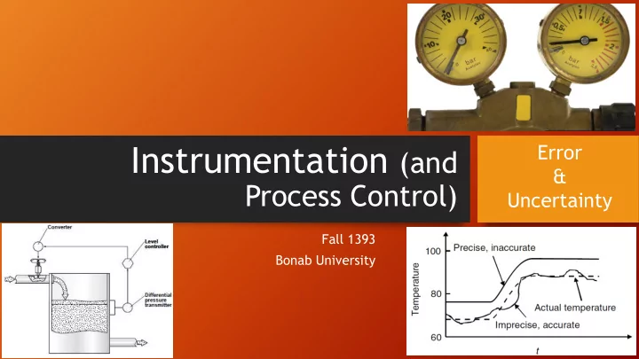
Instrumentation (and
Process Control)
Fall 1393 Bonab University
Measurement Uncertainty - Error & Uncertainty Measurement - - PowerPoint PPT Presentation
Instrumentation (and Error & Process Control) Uncertainty Fall 1393 Bonab University Error Measurement Uncertainty - Error & Uncertainty Measurement errors are impossible to avoid We can minimize their magnitude by Good
Fall 1393 Bonab University
2
Error & Uncertainty
reading, that is, either all errors are positive or are all negative
caused by random and unpredictable effects, such that positive errors and negative errors
3
Error & Uncertainty
system being measured
system disturbance is needed to minimize it
4
Error & Uncertainty
R1 = 400 O; R2 = 600 O; R3 = 1000 O; R4 = 500 O; R5 = 1000 O The voltage across AB is measured by a voltmeter whose internal resistance is 9500 O. What is the measurement error caused by the resistance of the measuring instrument?
RAB=500 measurement error = EO – Em = EO(1-9500/10000) = 0.05 EO 5%
5
Error & Uncertainty
particular environmental conditions
(a) a 0.9 kg rat in the box (real input) (b) an empty box with a 0.9 kg bias on the scale due to a temperature change (environmental input) (c) a 0.4 kg mouse in the box together with a 0.5 kg bias (real þ environmental inputs)
measured quantity (the real input) can be determined from the output reading of an instrument
6
Error & Uncertainty
instrument components
7
Error & Uncertainty
sources of error
environmental input that cancels it out
8
Error & Uncertainty
environmental input ( temperature change) will alter the value of the coil current for a given applied voltage alter the pointer output reading
where Rcomp has a temperature coefficient equal in magnitude but opposite in sign to that of the coil
9
Error & Uncertainty
, but changes with environment
high Ka
current-carrying cables
, BP , BS) reduces noise amplitude
10
Error & Uncertainty
11
Error & Uncertainty
12
Error & Uncertainty
systematic errors? quantify the maximum likely systematic error
rather a random error
basis for estimating the maximum likely error
13
Error & Uncertainty
14
Error & Uncertainty
error: sum of the separate errors = ±3%
estimate (manufacturer gives) about performance
frequency
15
Error & Uncertainty
(achievable in use)
included in the accuracy calculation in the manufacturer’s data sheet)
are estimated:
+1.2% (Xm-Xt)
0.5%
square method.
16
Error & Uncertainty
17
Error & Uncertainty Set Mean Median
A
398 420 394 416 404 408 400 420 396 413 430 409 408
B
409 406 402 407 405 404 407 404 407 407 408 406 407
C
409 406 402 407 405 404 407 404 407 407 408 406.5 406 406 410 406 405 408 406 409 406 405 409 406 407
confidence?
430-394=36 vs 409-402=7
to mean
examining distribution
18
Error & Uncertainty Set Mean Median spread
V σ
A
409 408 36 137 11.7
B
406 407 7 4.2 2.05
C
406.5 406 8 3.53 1.88
_ _
Random error symmetry
19
Error & Uncertainty
# Measurements
mm
particular shape that is called Gaussian
the frequency of large deviations
errors lie inside deviation boundaries of ±σ 68%
95.4%
99.7%
20
±1.96σ 95% (Very common)
Error & Uncertainty
mean
sets of measurements relative to the true mean = standard error of the mean α
predict the true value what is the likely error?
21
Error & Uncertainty
Mean of 10
predict the true value what is the likely error?
does not exceed |α|
22
Error & Uncertainty
Mean of 10
Not so good
23
Error & Uncertainty
24
Boxplot
Error & Uncertainty
25
Error & Uncertainty
and 330 in series)
26
Error & Uncertainty